WindMar Technical Documentation
Weather routing & performance analytics for merchant ships
| v0.1.0 | 2026-02-22 | Commercial compliance (CII, FuelEU Maritime, charter party tools, voyage reporting) + production optimizer (GSHHS coastline, 9 strait shortcuts, Pareto front, course-change penalty, safety fallback, A*-primary with optional VISIR) + security hardening (pickle RCE fix, input bounds, CORS, rate limits, NaN/Inf sanitization), ~67K LOC, 734 tests |
| v0.0.9 | 2026-02-20 | Modular architecture refactoring (6,922→281 LOC main.py, 9 domain routers, 37 Pydantic schemas), calibration improvements (ME-specific fuel, laden/ballast detection from ME load %, widened bounds), engine log deduplication, 426 tests passing |
| v0.0.8 | 2026-02-18 | Vessel model upgrade (SFOC calibration fix, Kwon + STAWAVE-1 dual wave methods, bisection performance predictor), engine log analytics (CSV/Excel upload, 5 KPIs, 6 charts, calibration bridge), weather pipeline refactoring (user-triggered overlays, viewport-aware resync, deferred supersede), Dijkstra cost formula fix (safety on fuel only), hard avoidance limits (Hs ≥ 6 m, wind ≥ 70 kts), dashboard layout harmonization, 79 API endpoints |
| v0.0.7 | 2026-02-13 | Two-mode architecture (Weather/Analysis), 7 weather layers with WMO color ramps, forecast timeline for all layers, analysis panel + detail page with per-waypoint passage plan, route save/load, current & wave direction in results, Monte Carlo P10/P50/P90, vessel speed sync |
| v0.0.6 | 2026-02-10 | ECDIS-style UI redesign, dual speed-strategy optimization (Same Speed / Match ETA), voyage baseline gating, wave crest rendering with polar diagram, GFS wind DB ingestion, turn-angle path smoothing |
| v0.0.5 | 2026-02-09 | Weather DB architecture, temporal weather provisioning, Monte Carlo with correlated perturbations, CII compliance, PostgreSQL persistence |
| v0.0.4 | 2026-02-09 | Frontend refactor, Monte Carlo simulation, grid weather provider |
| v0.0.3 | 2026-02-09 | Data sources docs, credential setup, modernize pyproject.toml |
| v0.0.2 | 2026-02-08 | GFS near-real-time wind data + 5-day forecast timeline |
| v0.0.1 | 2026-02-08 | Initial public release |
WindMar is a physics-based vessel performance modeling system with weather-aware A* route optimization, fuel consumption minimization, and IMO CII compliance tracking. It combines hydrodynamic resistance calculations, seakeeping analysis, and real-time weather data to find the safest and most fuel-efficient routes for merchant ships.
What is WindMar?
WindMar is an end-to-end maritime route optimization platform designed for Medium Range (MR) product tankers. It models the complete chain of vessel performance physics — from calm water resistance through wind and wave added resistance, engine SFOC curves, and propulsion efficiency — to predict fuel consumption under real weather conditions. The A* pathfinding algorithm then searches for the route that minimizes total fuel consumption while respecting safety constraints and regulatory zones. All calculations are grounded in established naval architecture methods: Holtrop-Mennen for hull resistance, Blendermann for wind loads, Kwon for wave added resistance, and simplified strip theory for seakeeping motions.
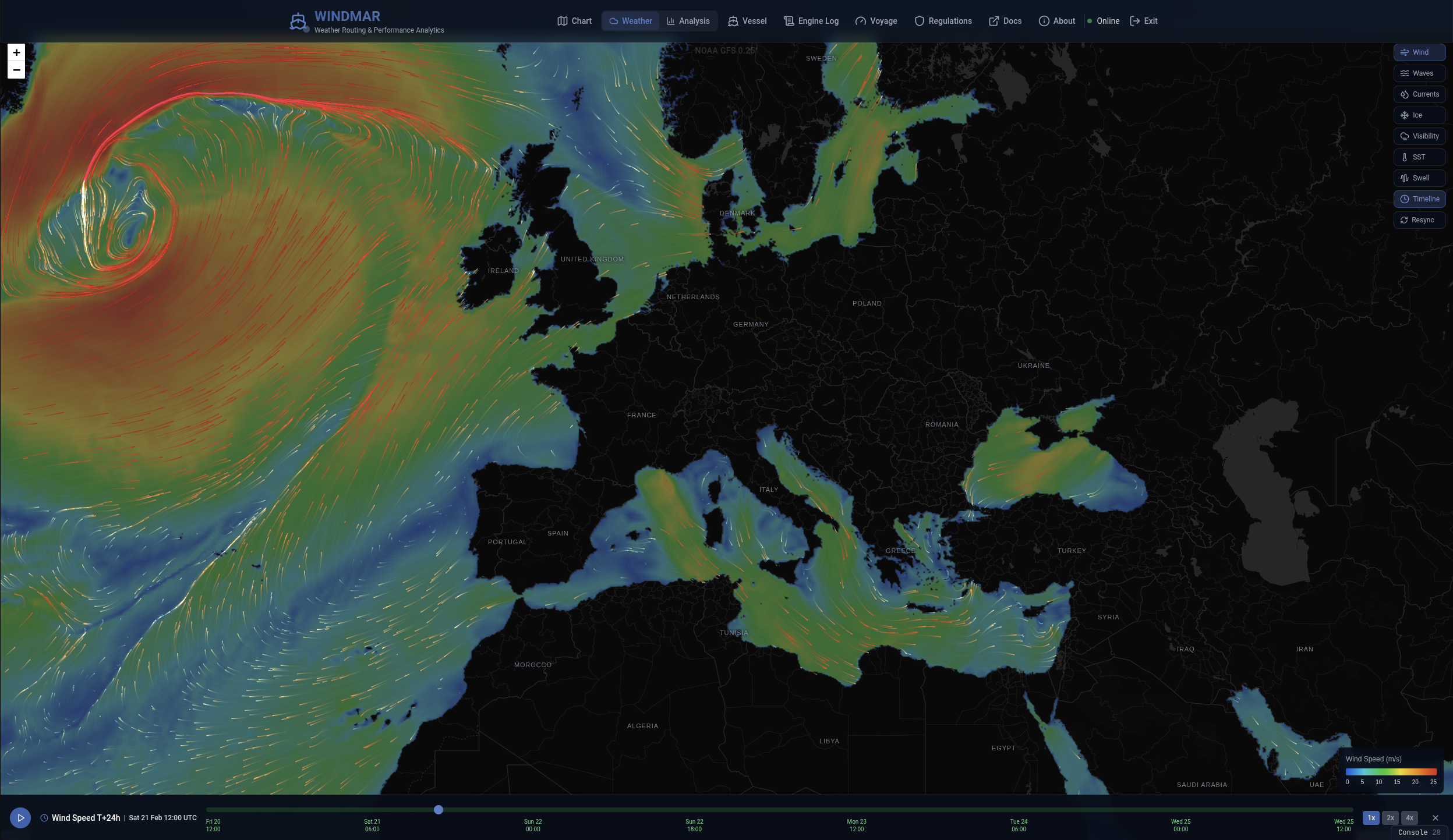
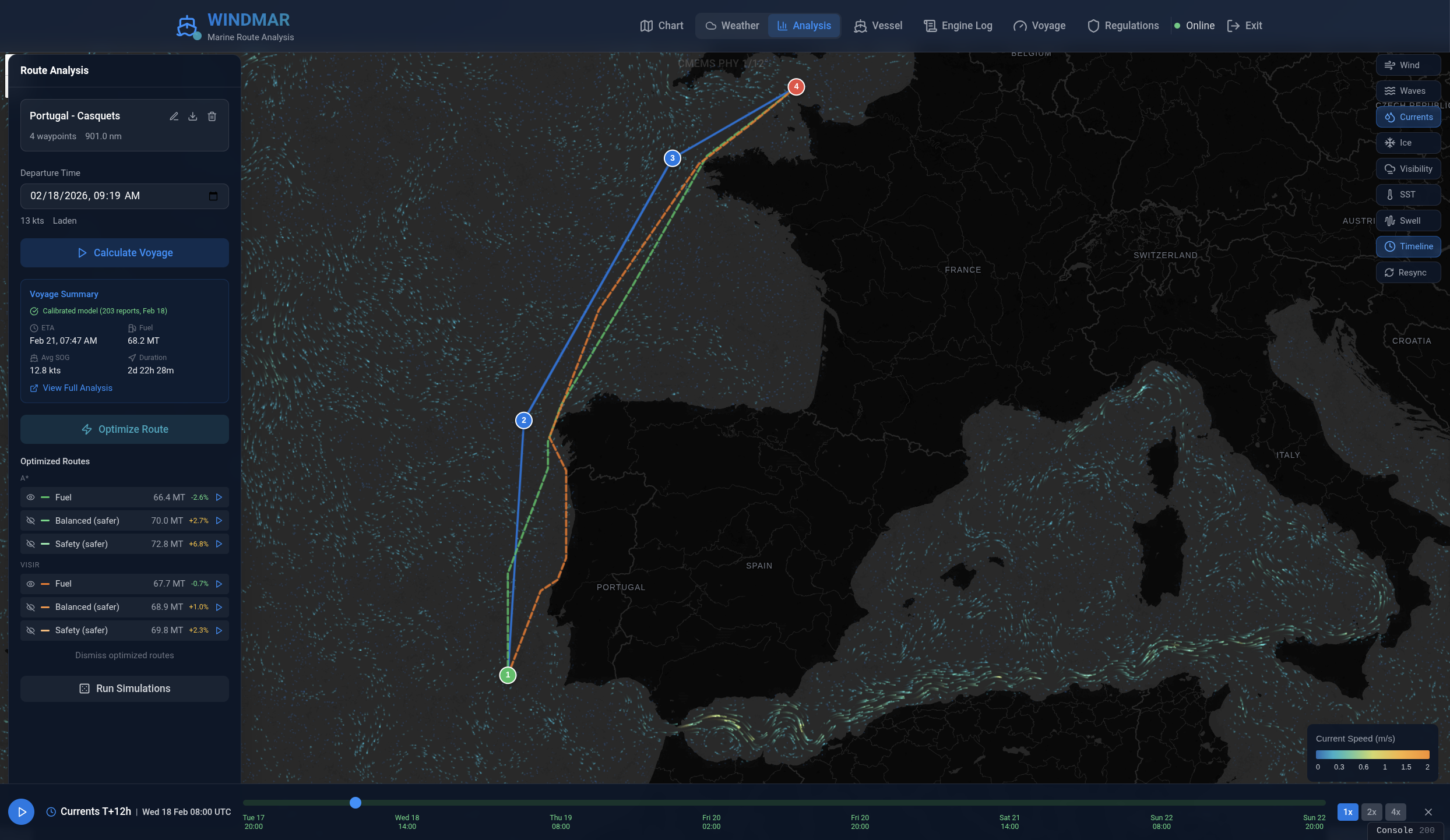
The system ingests near-real-time wind data from NOAA GFS (0.25° resolution, via NOMADS), wave, current, SST, swell, visibility, and ice data from Copernicus Marine Service (CMEMS), with ERA5 reanalysis as a secondary wind fallback. Weather grids are pre-ingested into PostgreSQL on a 6-hourly cycle (wind, waves, currents, ice), with on-demand prefetch for SST, visibility, and swell — enabling sub-second route calculations. A forecast timeline (f000–f120, 3-hourly steps) supports all 7 weather layers with play/pause and scrubbing. The interface uses a two-mode architecture: Weather mode presents a full-screen ECDIS-style chart with 7 weather overlays and WMO-standard color ramps; Analysis mode displays a left panel (320px) for route import, voyage calculation, optimization comparison (A* engine with optional VISIR Dijkstra), and Monte Carlo simulation (P10/P50/P90). A dedicated analysis page shows a per-waypoint passage plan with ETA, SOG, wind, waves, current speed/direction, fuel, and data source badges. The system evaluates vessel motions (roll, pitch, vertical acceleration) and enforces safety criteria that block or penalize dangerous sea states. It calculates the IMO Carbon Intensity Indicator (CII) rating for the completed voyage, enabling operators to assess regulatory compliance before departure.
Vessel Performance
- Holtrop-Mennen calm water resistance
- Blendermann wind resistance model
- Kwon wave added resistance formula
- Engine SFOC curves with load-dependent correction
Route Optimization
- A* grid search with 9 strait shortcuts (primary engine)
- 3 safety-weight variants + Pareto front (fuel vs. time)
- Course-change penalty, safety fallback routing
- Per-waypoint passage plan with SOG profile
Seakeeping Safety
- Roll, pitch, and acceleration prediction
- Slamming probability assessment
- Parametric roll risk detection
- Safety constraints in route optimization
Weather Integration
- 7 layers: wind, waves, currents, swell, SST, visibility, ice
- Forecast timeline for all layers (5-day, 3h steps)
- WMO-standard color ramps per field
- 6-hourly DB ingestion + on-demand prefetch
IMO Compliance
- CII rating calculator (A through E)
- MEPC.339(76) reference values
- Multi-year reduction factor projections
- CO2 emission factors for multiple fuel types
Vessel Calibration
- Noon report processing from Excel
- scipy.optimize parameter fitting
- Per-component calibration factors
- RMSE-based objective minimization
Architecture
Component Overview
WindMar follows a layered architecture with a clear separation between the user-facing frontend, the API backend, the physics-based optimization engine, and external data providers. Each component runs as an independent service orchestrated via Docker Compose.
| Component | Technology | Responsibility |
|---|---|---|
| Frontend | Next.js 15 | Two-mode UI (Weather/Analysis), 7 weather map layers, route analysis panel, passage plan |
| Backend | FastAPI (Python) | REST API, request validation, orchestration of optimization engine |
| Optimization Engine | Python (NumPy, SciPy) | Physics models, A* pathfinding, speed optimization, seakeeping |
| Weather Provider | NOAA GFS / CMEMS / ERA5 | GFS wind, CMEMS waves/currents/SST/swell/visibility/ice, ERA5 fallback, 5-day forecast |
| Database | PostgreSQL 16 | Vessel specs, route history, calibration data, regulatory zones |
| Cache | Redis 7 / In-memory | Rate limiting, session state; weather fields cached in-memory |
Data Flow
- Route Definition — User defines departure, arrival, and waypoints on the map interface. Vessel condition (laden/ballast) and speed preferences are selected.
- Weather Fetch — Backend requests weather data from Copernicus for the route corridor. Wind, wave, and current fields are interpolated to the optimization grid.
- Performance Calculation — For each grid cell, the optimization engine computes total resistance (calm water + wind + waves), brake power, SFOC, and fuel consumption at candidate speeds.
- A* Pathfinding — The A* algorithm searches the grid using fuel consumption as the edge cost. Safety constraints block or penalize dangerous cells. Regulatory zones modify costs.
- Speed Optimization — Each leg of the optimal path is individually speed-optimized to minimize fuel per nautical mile given local weather conditions.
- Results — The optimized route, fuel estimate, ETA, leg-by-leg breakdown, seakeeping assessment, and CII rating are returned to the frontend for display.
Docker Services
services:
  db:
    image: postgres:16-alpine
    ports: ["${DB_PORT:-5432}:5432"]

  redis:
    image: redis:7-alpine
    ports: ["${REDIS_PORT:-6379}:6379"]

  api:
    build: .
    ports: ["${API_PORT:-8000}:8000"]
    depends_on: [db, redis]

  frontend:
    build: ./frontend
    ports: ["${FRONTEND_PORT:-3000}:3000"]
    depends_on: [api]
All ports and credentials are configured via environment variables in .env
(see .env.example for defaults). Copy and customize before starting.
Installation
Prerequisites
- Python 3.10 or later
- Node.js 18 or later
- Docker & Docker Compose
Docker Compose (Recommended)
git clone https://github.com/windmar-nav/windmar.git
cd windmar
cp .env.example .env    # Edit with your settings
docker compose up -d --build
This starts all four services (PostgreSQL, Redis, API, frontend). By default the frontend is accessible
at http://localhost:3000 and the backend API at http://localhost:8000.
Ports are configurable via .env.
Manual Setup
Backend
pip install -r requirements.txt
python api/main.py
Frontend
cd frontend
npm install --legacy-peer-deps
npm run dev
Weather Data Sources
WindMar uses a three-tier provider chain that automatically falls back when a source is unavailable. See Weather Data Acquisition for full technical details.
| Data Type | Primary Source | Fallback | Credentials |
|---|---|---|---|
| Wind | NOAA GFS (0.25°) | ERA5 → Synthetic | None (free) |
| Waves | CMEMS wave model | Synthetic | CMEMS account |
| Currents | CMEMS physics model | Synthetic | CMEMS account |
| Forecast | GFS f000–f120 (5-day) | — | None |
Obtaining Weather Credentials
CMEMS (waves and currents): Register at
marine.copernicus.eu,
then set in .env:
COPERNICUSMARINE_SERVICE_USERNAME=your_username
COPERNICUSMARINE_SERVICE_PASSWORD=your_password
CDS ERA5 (wind fallback): Register at cds.climate.copernicus.eu, copy your Personal Access Token from your profile, then set:
CDSAPI_KEY=your_personal_access_tokenEnvironment Variables
Copy .env.example to .env and configure. Key variables:
DATABASE_URL=postgresql://windmar:password@db:5432/windmar
REDIS_URL=redis://:password@redis:6379/0
API_SECRET_KEY=generate_with_openssl_rand_hex_32
COPERNICUSMARINE_SERVICE_USERNAME=your_username
COPERNICUSMARINE_SERVICE_PASSWORD=your_password
CDSAPI_KEY=your_cds_personal_access_tokenNever commit
.env to version control. The .gitignore excludes it by default.
See .env.example for all available variables with descriptions.
Tech Stack
Backend
| Library | Version | Purpose |
|---|---|---|
| FastAPI | 0.104+ | REST API framework |
| Uvicorn | 0.24+ | ASGI server |
| SQLAlchemy | 2.0+ | ORM and database access |
| Pydantic | 2.0+ | Request/response validation |
| Alembic | 1.13+ | Database migrations |
Frontend
| Library | Version | Purpose |
|---|---|---|
| Next.js | 15 | React framework with SSR |
| React | 19 | UI component library |
| Leaflet | 1.9+ | Map rendering and route display |
| Recharts | 2.10+ | Charts for fuel, CII, seakeeping data |
| Tailwind CSS | 3.4+ | Utility-first styling |
Scientific Computing
| Library | Version | Purpose |
|---|---|---|
| NumPy | 1.26+ | Array operations, vector math |
| SciPy | 1.11+ | Optimization (Nelder-Mead), interpolation |
| global-land-mask | 1.0+ | Land/ocean grid classification |
| xarray | 2024.1+ | NetCDF weather data handling |
| copernicusmarine | 1.0+ | Copernicus CMEMS API client |
Database & Cache
| Service | Version | Purpose |
|---|---|---|
| PostgreSQL | 16 | Persistent storage for vessel specs, routes, zones |
| Redis | 7 | Weather field caching, session state |
External APIs
| Service | Data | Resolution |
|---|---|---|
| Copernicus CMEMS | Significant wave height, wave period, wave direction | 0.25 deg, 3-hourly |
| ERA5 Reanalysis | 10m wind speed, wind direction | 0.25 deg, hourly |
| Copernicus CMEMS | Ocean current speed and direction | 0.083 deg, daily |
Calm Water Resistance
Calm water resistance is the foundation of all fuel consumption predictions. WindMar implements the Holtrop-Mennen method, the industry-standard empirical approach for estimating hull resistance of displacement vessels. The method decomposes total resistance into frictional, wave-making, and appendage components, each derived from the vessel's principal dimensions and hull form coefficients.
Holtrop-Mennen Method
Where:
- \(R_f\) = Frictional resistance (dominant at low Froude numbers)
- \(R_w\) = Wave-making resistance (grows exponentially with speed)
- \(R_{\text{app}}\) = Appendage resistance (rudder, shaft brackets, etc.)
A) Frictional Resistance (R_f)
Frictional resistance arises from the viscous shear stress between the hull surface and the surrounding water. It dominates at service speeds typical of MR tankers (Froude number 0.12-0.18). The ITTC 1957 model-ship correlation line provides the friction coefficient, and the Holtrop form factor accounts for the three-dimensional shape of the hull.
Where:
- \(\rho_{sw} = 1025 \; \text{kg/m}^3\) (seawater density)
- \(V\) = ship speed (m/s)
- \(S\) = wetted surface area (m²)
- \(C_f = \frac{0.075}{(\log_{10} Re - 2)^2}\) (ITTC 1957 friction line)
- \(Re = \frac{V \cdot L_{pp}}{\nu_{sw}}\) (Reynolds number)
- \(\nu_{sw} = 1.19 \times 10^{-6} \; \text{m}^2\text{/s}\) (kinematic viscosity at 15°C)
At service speed of 13 knots (6.69 m/s) with L_pp = 176 m, the Reynolds number is approximately 9.9 × 10⁸, placing the flow firmly in the turbulent regime. The friction coefficient C_f is then approximately 0.00148.
Form Factor (1 + k_1)
The form factor corrects the flat-plate friction coefficient for the three-dimensional hull shape. Holtrop-Mennen provides a regression formula for tanker hull forms based on the principal dimension ratios and block coefficient.
Default MR tanker values:
- \(B / L_{pp} = 32 / 176 = 0.182\)
- \(B / T_{\text{laden}} = 32 / 11.8 = 2.71\)
- \(B / T_{\text{ballast}} = 32 / 6.5 = 4.92\)
- \(C_{b,\text{laden}} = 0.82\)
- \(C_{b,\text{ballast}} = 0.75\)
Resulting form factors:
- \((1 + k_1)_{\text{laden}} = 1 + 0.93 + 0.4871 \times 0.182 - 0.2156 \times 2.71 + 0.1027 \times 0.82 \approx 1.52\)
- \((1 + k_1)_{\text{ballast}} \approx 1.35\)
B) Wave-Making Resistance (R_w)
Wave-making resistance is generated by the pressure field around the hull that creates surface waves. For MR tankers operating at low Froude numbers (Fr < 0.2), wave-making resistance is a small fraction of total resistance. However, it increases exponentially with speed, making it the dominant factor limiting maximum speed.
Where:
- \(Fr = \frac{V}{\sqrt{g \cdot L_{pp}}}\) (Froude number)
- \(c_1 = 2223105 \cdot C_b^{3.78613} \cdot (T/B)^{1.07961}\)
- \(c_7 = 0.229577 \cdot (B/L_{pp})^{1/3}\)
- \(\Delta\) = displacement (tonnes)
- \(g = 9.81 \; \text{m/s}^2\)
At the design speed of 13 knots, the Froude number for an MR tanker is approximately Fr = 6.69 / sqrt(9.81 × 176) ≈ 0.161. The exponential term exp(-0.4 × 0.161-2) is very small, confirming that wave-making resistance contributes less than 5% of total resistance at service speed.
C) Appendage Resistance (R_app)
Appendage resistance accounts for the drag of the rudder, propeller shaft brackets, bilge keels, and other hull appendages. For MR tankers with standard appendage configurations, this is estimated as a fixed percentage of frictional resistance.
Default MR Tanker Specifications
| Parameter | Laden | Ballast |
|---|---|---|
| LOA | 183.0 m | 183.0 m |
| L_pp | 176.0 m | 176.0 m |
| Beam | 32.0 m | 32.0 m |
| Draft | 11.8 m | 6.5 m |
| Displacement | 65,000 MT | 20,000 MT |
| Block Coefficient (C_b) | 0.82 | 0.75 |
| Wetted Surface | 7,500 m² | 5,200 m² |
| Service Speed | 13.0 kts | 13.0 kts |
| DWT | 49,000 MT | — |
| MCR | 6,600 kW | 6,600 kW |
| SFOC at MCR | 171 g/kWh | 171 g/kWh |
Wind Resistance
Wind resistance is computed using the Blendermann method, which models the aerodynamic forces on the vessel's above-water structure as a function of relative wind speed, direction, and the vessel's projected areas. The method accounts for both longitudinal (drag) and transverse (side force) components, with the longitudinal component directly opposing forward motion and the transverse component contributing indirectly through induced drift.
Blendermann Method
Range: \(0°\) (head wind) to \(180°\) (following wind)
Longitudinal coefficient:
\[C_x = -0.6 \cdot \cos(\theta_{\text{rel}}) + 0.8 \cdot \cos^2(\theta_{\text{rel}})\]Transverse coefficient:
\[C_y = 0.9 \cdot \sin(\theta_{\text{rel}})\]Longitudinal force:
\[F_x = \tfrac{1}{2} \cdot \rho_{\text{air}} \cdot V_{\text{wind}}^2 \cdot A_{\text{frontal}} \cdot |C_x|\]Transverse force:
\[F_y = \tfrac{1}{2} \cdot \rho_{\text{air}} \cdot V_{\text{wind}}^2 \cdot A_{\text{lateral}} \cdot |C_y|\]Total wind resistance:
\[R_{\text{wind}} = F_x + 0.1 \cdot F_y\]Where:
- \(\rho_{\text{air}} = 1.225 \; \text{kg/m}^3\) (air density at 15°C, sea level)
- \(V_{\text{wind}}\) = true wind speed (m/s)
- \(A_{\text{frontal}}\) = projected frontal area (m²)
- \(A_{\text{lateral}}\) = projected lateral area (m²)
Wind Projection Areas
| Area | Laden | Ballast |
|---|---|---|
| Frontal (A_frontal) | 450 m² | 850 m² |
| Lateral (A_lateral) | 2,100 m² | 2,800 m² |
In ballast condition the vessel rides higher, exposing 89% more frontal area (850 vs 450 m²) and 33% more lateral area (2,800 vs 2,100 m²) to the wind. This results in significantly higher windage forces, particularly in head wind conditions where ballast wind resistance can exceed laden resistance by a factor of two or more.
Physical Interpretation by Wind Angle
- Head wind (0°) — Maximum longitudinal resistance. C_x reaches its peak value. This is the worst-case scenario for fuel consumption.
- Beam wind (90°) — Minimal longitudinal component but maximum transverse force. The 10% coupling factor from F_y captures the drift-induced resistance.
- Following wind (180°) — Minimal resistance. The wind partially assists forward motion. C_x is near zero or slightly negative (assisting).
Wave Resistance
Wave added resistance is the increase in hull resistance caused by the vessel's interaction with ocean waves. WindMar uses the Kwon empirical formula, which estimates added resistance as a function of significant wave height, beam, Froude number, and the encounter angle between the vessel heading and the dominant wave direction.
Kwon Empirical Formula
Directional factor:
\[f_{\text{dir}} = \frac{1 + \cos(\theta_{\text{encounter}})}{2}\]Values by encounter angle:
- Head seas (\(\theta = 0°\)): \(f_{\text{dir}} = 1.0\)
- Bow quarter (\(\theta = 45°\)): \(f_{\text{dir}} = 0.85\)
- Beam seas (\(\theta = 90°\)): \(f_{\text{dir}} = 0.5\)
- Stern quarter (\(\theta = 135°\)): \(f_{\text{dir}} = 0.15\)
- Following seas (\(\theta = 180°\)): \(f_{\text{dir}} = 0.0\)
Where:
- \(H_s\) = significant wave height (m)
- \(B\) = beam (m)
- \(Fr = \frac{V}{\sqrt{g \cdot L_{pp}}}\) (Froude number)
- \(\rho_{sw} = 1025 \; \text{kg/m}^3\)
- \(g = 9.81 \; \text{m/s}^2\)
The Kwon formula produces a quadratic dependence on wave height: doubling H_s from 2 m to 4 m increases wave added resistance by a factor of four. The directional factor ensures that head seas produce maximum added resistance while following seas produce none, which matches the physical expectation that waves opposing the vessel's motion cause the greatest speed loss.
Dual Wave Method (v0.0.8)
Since v0.0.8, WindMar supports two wave added resistance methods, selectable via the
wave_method parameter on the vessel model:
stawave1(default) — ISO 15016 STAWAVE-1 method. A simplified, internationally standardized formula that estimates wave added resistance from significant wave height, vessel length, beam, and block coefficient. Well-suited for sea trial corrections and regulatory compliance calculations.kwon— Kwon empirical method (documented above). Estimates speed loss percentage from wave height, vessel particulars, and encounter angle. More physically detailed directional response; well-validated for merchant vessels at service speed.
Both methods are available via the POST /api/vessel/predict endpoint. The active method
is reported by GET /api/vessel/model-status.
For a laden MR tanker in head seas with H_s = 3 m at service speed (Fr ≈ 0.161), the wave added resistance is approximately:
SFOC Curve
Specific Fuel Oil Consumption (SFOC) describes the mass of fuel consumed per unit of energy delivered by the engine. It varies with engine load: marine diesel engines have an optimal efficiency zone around 75% of Maximum Continuous Rating (MCR), with increasing specific consumption at both lower and higher loads. WindMar models this behavior with a piecewise linear correction applied to the MCR reference SFOC.
Below optimal load (\(l_f < 0.75\)):
\[\text{SFOC} = \text{SFOC}_{MCR} \times \bigl(1.0 + 0.15 \times (0.75 - l_f)\bigr)\]At or above optimal load (\(l_f \ge 0.75\)):
\[\text{SFOC} = \text{SFOC}_{MCR} \times \bigl(1.0 + 0.05 \times (l_f - 0.75)\bigr)\]Constraints:
- \(l_f = \max\bigl(0.15,\; \min(1.0,\; P_{\text{brake}} / P_{MCR})\bigr)\)
- \(\text{SFOC}_{MCR} = 171 \; \text{g/kWh}\) (manufacturer specification)
The asymmetric correction reflects the physical reality of diesel engine combustion: at low loads, incomplete combustion and thermal losses increase specific consumption more steeply (15% penalty per 0.1 load fraction below 75%) than the mild increase at high loads (5% penalty per 0.1 above 75%) caused by increased cylinder pressures and thermal stress.
SFOC Behavior by Engine Load
| Engine Load | SFOC (g/kWh) | Efficiency Note |
|---|---|---|
| 15% (minimum) | ~186 | Minimum load limit; high specific consumption |
| 50% | ~177 | Part-load penalty; below optimal range |
| 75% | ~171 | Optimal operating point; minimum SFOC |
| 85% | ~172 | Near optimal; slight overload penalty |
| 100% (MCR) | ~173 | Full load; mild thermal penalty |
The engine load is clamped to the range [0.15, 1.0]. Below 15% load, the engine is considered non-operational. Above 100% MCR, the engine cannot deliver more power, so the brake power is capped at P_MCR = 8,840 kW.
SFOC Calibration Factor (v0.0.8)
Since v0.0.8, the SFOC curve supports a multiplicative calibration factor (sfoc_factor)
derived from engine log analysis. When the vessel is calibrated from actual noon report or engine log
data, the optimizer may determine that the manufacturer's SFOC reference is over- or under-estimated.
The corrected SFOC is:
Where:
- \(k_{\text{sfoc}}\) = SFOC calibration factor (default 1.0, typically 0.9–1.15)
- \(\text{SFOC}(l_f)\) = uncalibrated piecewise curve from above
The factor is stored alongside the hull calibration factors (calm_water,
wind, waves) and is applied globally to all fuel consumption
calculations, route optimization, and CII compliance estimates. It is set via
POST /api/vessel/calibrate or POST /api/engine-log/calibrate.
Propulsion Chain
The propulsion chain converts total hull resistance into brake power demand and then into fuel consumption. It accounts for the efficiencies of the propeller, the hull-propeller interaction, and the relative rotative efficiency of the propulsion system.
Brake Power Calculation
Tow power (power to overcome resistance):
\[P_{\text{tow}} = \frac{R_{\text{total}} \cdot V}{1000} \quad [\text{kW}]\]Where:
- \(R_{\text{total}} = R_{\text{calm}} + R_{\text{wind}} + R_{\text{wave}}\) [N]
- \(V\) = ship speed [m/s]
Brake power (engine output):
\[P_{\text{brake}} = \frac{P_{\text{tow}}}{\eta_{\text{prop}} \cdot \eta_{\text{hull}} \cdot \eta_{\text{rre}}}\]Where:
- \(\eta_{\text{prop}} = 0.65\) (propeller open-water efficiency)
- \(\eta_{\text{hull}} = 1.05\) (hull efficiency; > 1 due to wake gain)
- \(\eta_{\text{rre}} = 1.00\) (relative rotative efficiency)
Combined propulsive efficiency:
\[\eta_{\text{total}} = \eta_{\text{prop}} \cdot \eta_{\text{hull}} \cdot \eta_{\text{rre}} = 0.65 \times 1.05 \times 1.00 = 0.6825\]Power capped at MCR:
\[P_{\text{brake}} = \min(P_{\text{brake}},\; P_{MCR}) \quad \text{where } P_{MCR} = 8{,}840 \; \text{kW}\]Hull efficiency exceeds 1.0 because the wake behind the hull reduces the effective inflow velocity to the propeller relative to the ship speed. The propeller operates in a flow field that is slower than the free-stream velocity, requiring less thrust to overcome the same resistance.
Fuel Consumption
Where:
- \(P_{\text{brake}}\) = brake power [kW]
- \(\text{SFOC}\) = specific fuel oil consumption [g/kWh] (load-dependent)
- \(t_{\text{hours}}\) = duration of the leg [hours]
- \(1{,}000{,}000\) = conversion from grams to metric tonnes
For example, at service speed in calm water with P_brake = 5,500 kW and SFOC = 172 g/kWh, a 24-hour transit consumes approximately:
Fuel = (5500 × 172 × 24) / 1,000,000 = 22.7 MT/dayShip Motions
Ship motion prediction is essential for seakeeping assessment and safety enforcement during route optimization. WindMar implements simplified strip-theory models for roll, pitch, and vertical acceleration. These models provide physically meaningful motion estimates that capture the dominant effects of wave height, encounter frequency, and vessel loading condition.
Roll Motion — Single DOF Oscillator
Roll is modeled as a single degree-of-freedom oscillator driven by the transverse wave slope. The response amplitude operator (RAO) captures the frequency-dependent magnification, with resonance occurring when the encounter frequency matches the vessel's natural roll frequency.
Roll amplitude [rad]:
\[\phi = \frac{\text{wave\_slope}}{GM} \cdot \frac{H_s}{2} \cdot \text{RAO} \cdot \sin(\theta_{\text{beam}})\]Response Amplitude Operator:
\[\text{RAO} = \frac{1}{\sqrt{\left(1 - \left(\frac{\omega_e}{\omega_{\text{roll}}}\right)^2\right)^2 + \left(2 \zeta \cdot \frac{\omega_e}{\omega_{\text{roll}}}\right)^2}}\]Where:
- \(\omega_{\text{roll}} = \frac{2\pi}{T_{\text{roll}}}\) (natural roll frequency)
- \(T_{\text{roll}}\): 14 s (laden), 10 s (ballast)
- \(\zeta = 0.05\) (5% critical damping)
- \(GM\): 2.5 m (laden), 4.0 m (ballast)
- \(\theta_{\text{beam}}\) = angle from beam (90° = pure beam seas)
- \(\omega_e\) = encounter frequency (depends on ship speed & heading)
The natural roll period is longer in laden condition (14 s) due to the higher metacentric height combined with greater mass moment of inertia. Ballast condition has a shorter period (10 s) because the higher GM (4.0 m) produces a stiffer restoring moment relative to the reduced inertia. The 5% critical damping ratio is conservative and accounts for hull friction, bilge keel effects, and cargo damping.
Pitch Motion
Pitch is driven primarily by head seas and bow-quarter seas. The amplitude depends on the wave slope, the encounter angle (maximum in head seas), and a pitch factor that captures the wavelength-to-ship-length tuning effect.
Pitch amplitude [deg]:
\[\theta_{\text{pitch}} = 10 \cdot \text{wave\_slope} \cdot |\cos(\theta_{\text{enc}})| \cdot f_{\text{pitch}}\]Pitch factor depends on \(L/\lambda\) ratio:
\[f_{\text{pitch}} = \begin{cases} 2 \cdot (L / \lambda) & L/\lambda < 0.5 \\ 1 - 0.3 \cdot |L/\lambda - 1| & 0.5 \le L/\lambda < 1.5 \\ 0.5 / (L / \lambda) & L/\lambda \ge 1.5 \end{cases}\]Where:
- \(\lambda = \frac{g \cdot T_{\text{wave}}^2}{2\pi}\) (deep water wavelength)
- \(L = L_{pp} = 176 \; \text{m}\)
- \(T_{\text{wave}}\) = peak wave period (s)
The pitch factor peaks near L/λ = 1 (ship length equals wavelength), where the vessel "straddles" consecutive wave crests and troughs, producing maximum pitching motion. When the wavelength is much shorter or longer than the ship, the pitch factor decreases because the vessel either averages out multiple short waves or rides on a single long wave slope.
Vertical Acceleration
Vertical acceleration at specific locations along the ship length combines the heave acceleration at the center of gravity with the pitch-induced acceleration component. Points far from midship (bridge, bow) experience amplified accelerations due to the pitch lever arm.
Heave acceleration (at center of gravity):
\[a_{\text{heave}} = \frac{H_s}{2} \cdot \omega_e^2 \cdot \bigl(0.3 + 0.7 \cdot \cos(\theta_{\text{enc}})\bigr)\]Point acceleration (at distance \(x\) from midship):
\[a_{\text{point}} = \sqrt{a_{\text{heave}}^2 + \bigl(x \cdot \theta_{\text{pitch,rad}} \cdot \omega_e^2\bigr)^2}\]Reference locations:
- Bridge: \(x = -70\) m from midship (aft)
- Bow: \(x = +88\) m from midship (forward)
- Midship: \(x = 0\) m (minimum acceleration)
The bow experiences the highest vertical accelerations because it is the farthest point forward from the pitch axis. At the bridge (70 m aft of midship), accelerations are also amplified but less than at the bow. Vertical acceleration is the primary crew comfort criterion and drives speed reduction decisions in heavy weather.
Safety Criteria
WindMar enforces safety at two levels: hard avoidance limits that instantly reject extreme conditions, and a three-tier motion-based classification (Safe, Marginal, Dangerous) computed from the seakeeping model. Both are applied during route optimization by the A* engine (and VISIR Dijkstra when enabled).
Hard Avoidance Limits (v0.0.8)
These absolute thresholds are checked before computing vessel motions. Any grid cell exceeding either limit is assigned infinite cost — the optimizer cannot route through it regardless of heading or speed. These values are calibrated for an MR Product Tanker (~50k DWT).
| Parameter | Threshold | Equivalent |
|---|---|---|
| Significant wave height (Hs) | ≥ 6.0 m | Beaufort 9+ (severe gale) |
| Wind speed | ≥ 70 kts | Beaufort 12 (hurricane force) |
Motion-Based Safety Limits
| Motion Parameter | Safe | Marginal | Dangerous |
|---|---|---|---|
| Roll amplitude | < 15° | 15° – 25° | > 25° |
| Pitch amplitude | < 5° | 5° – 8° | > 8° |
| Vertical acceleration | < 0.2g | 0.2g – 0.3g | > 0.3g |
| Slamming probability | < 3% | 3% – 10% | > 10% |
Safety criteria are enforced by the routing engines. Grid cells classified as Dangerous receive a graduated penalty (2× to 5× cost, or infinite above 1.5× the dangerous threshold). Marginal cells receive a penalty proportional to the exceedance above safe limits. Safe cells use the nominal fuel-based cost. In both engines, safety penalties apply to fuel cost only — the time penalty remains unweighted to prevent artificial inflation of detour costs.
The overall safety classification for a cell is determined by the worst-case criterion: if any single parameter falls in the Dangerous range, the cell is classified as Dangerous regardless of the other parameters.
Slamming & Parametric Roll
Slamming (Ochi Criteria)
Slamming occurs when the bow emerges from the water and re-enters with high velocity, generating impulsive loads on the hull structure. The Ochi criteria estimate the probability of slamming based on bow emergence and re-entry velocity. Slamming risk is highest in ballast condition (lower forward draft) and head seas.
Where:
- \(H_s\) = significant wave height (m)
- \(L_{fp}\) = distance from midship to forward perpendicular (m)
- \(\theta_{\text{pitch}}\) = pitch amplitude (rad)
Emergence probability:
\[P_{\text{emergence}} = f(y_{\text{bow}},\; \text{freeboard})\]When \(y_{\text{bow}}\) exceeds bow freeboard, the bow emerges from the water and slamming becomes possible on re-entry.
Re-entry velocity:
\[v_{\text{impact}} = \sqrt{2 \cdot g \cdot \max(0,\; y_{\text{bow}} - \text{freeboard})}\]Where:
- \(g = 9.81 \; \text{m/s}^2\)
- freeboard = distance from waterline to deck at bow (m)
- Laden: freeboard \(\approx 5.2\) m
- Ballast: freeboard \(\approx 10.5\) m (higher deck but lower draft = more emergence)
Despite the higher freeboard in ballast, the reduced forward draft means the keel rises above the still water surface more frequently, particularly in head seas. The combination of high emergence amplitude and significant re-entry velocity produces the impulsive slamming loads that can cause structural damage to the forward hull plating.
Parametric Roll Risk
Parametric rolling is a dangerous phenomenon where roll amplitudes build up rapidly due to periodic variation in the vessel's waterplane area (and thus stability) as waves pass along the hull. It occurs primarily in head or following seas when the wave encounter period is approximately twice the natural roll period.
Parametric roll risk is elevated when:
- Encounter period ratio: \(\frac{T_{\text{wave}}}{T_{\text{roll}}} \approx 2.0\) (tolerance: \(1.8 < T_{\text{wave}}/T_{\text{roll}} < 2.2\))
- Wave height exceeds critical threshold: \(H_s > H_{\text{critical}}\)
- Head seas or following seas: \(\theta_{\text{encounter}} < 30°\) or \(\theta_{\text{encounter}} > 150°\)
When all three conditions are met, the route cell is flagged for elevated parametric roll risk.
Parametric roll can develop in just a few wave cycles, reaching amplitudes of 30–40 degrees or more. It is particularly dangerous because it can occur in moderate sea states where other motion criteria appear safe. Detection and avoidance through route optimization is a key safety feature.
A* Algorithm
Route optimization uses the A* pathfinding algorithm to find the minimum-cost path through a weather-dependent grid. Each grid cell has a traversal cost determined by the fuel consumption required to cross it at the locally optimal speed, considering all resistance components and safety constraints.
Grid Construction
- Resolution: Configurable, default 0.5 degrees (~30 nm at the equator)
- Land masking: Land cells are removed using the
global-land-masklibrary, which provides a 1-km resolution land/ocean classification - Corridor: The search grid extends ±5 degrees latitude and longitude around the direct great-circle route to limit search space while allowing sufficient deviation for weather routing
- Connectivity: 8-connected grid (cardinal + diagonal neighbors)
A* Search
Where:
- \(f(n)\) = total estimated cost of path through node \(n\)
- \(g(n)\) = actual cost from start to node \(n\) (accumulated fuel consumption)
- \(h(n)\) = heuristic estimate of cost from node \(n\) to goal
Heuristic:
\[h(n) = d_{\text{goal}} \times r_{\text{fuel,min}}\](admissible: never overestimates actual cost)
Move cost (node \(m\) to neighbor \(n\)):
\[\text{cost}(m, n) = \text{fuel\_consumption}(m, n, V_{\text{optimal}})\]Where fuel_consumption accounts for:
- Calm water resistance (Holtrop-Mennen)
- Wind resistance (Blendermann) at local wind conditions
- Wave resistance (Kwon) at local wave conditions
- Engine SFOC at resulting load
- Safety penalty multiplier (\(1.0\times\) safe, \(1.5\times\) marginal, \(\infty\) dangerous)
Diagonal cost:
\[\text{cost}_{\text{diagonal}} = \sqrt{2} \times \text{cost}_{\text{cardinal}}\]Search Procedure
- Initialize priority queue (min-heap ordered by f-score) with start node
- Pop node with lowest f-score
- If goal reached, reconstruct path and return
- For each of 8 neighbors:
- Skip if land cell or already visited with lower cost
- Compute weather at neighbor location (interpolated from grid)
- Compute fuel cost to traverse cell at optimal speed
- Apply safety and regulatory zone multipliers
- Update neighbor's g-score if new path is cheaper
- Add to priority queue
- Terminate if cells explored exceeds 50,000 (safety limit)
Cost Calculation Code
def compute_cell_cost(self, from_cell, to_cell, weather):
    """Compute fuel cost to traverse a grid cell."""
    distance_nm = haversine(from_cell.lat, from_cell.lon,
                            to_cell.lat, to_cell.lon)

    # Find optimal speed for this cell
    best_fuel = float('inf')
    best_speed = self.vessel.service_speed

    for speed_kts in np.linspace(6.0, 18.0, 7):
        speed_ms = speed_kts * 0.5144

        # Total resistance
        r_calm = self.vessel.calm_water_resistance(speed_ms)
        r_wind = self.vessel.wind_resistance(
            speed_ms, weather.wind_speed, weather.wind_dir,
            self.heading)
        r_wave = self.vessel.wave_resistance(
            speed_ms, weather.wave_height, weather.wave_dir,
            self.heading)
        r_total = r_calm + r_wind + r_wave

        # Brake power and fuel
        p_tow = r_total * speed_ms / 1000
        p_brake = min(p_tow / self.vessel.eta_total,
                      self.vessel.mcr)
        sfoc = self.vessel.sfoc(p_brake / self.vessel.mcr)
        time_h = distance_nm / speed_kts
        fuel_mt = p_brake * sfoc * time_h / 1e6

        if fuel_mt < best_fuel:
            best_fuel = fuel_mt
            best_speed = speed_kts

    # Apply safety multiplier
    safety = self.assess_safety(weather, best_speed)
    if safety == 'dangerous':
        return float('inf')
    elif safety == 'marginal':
        best_fuel *= 1.5

    return best_fuel
Path Smoothing
After A* finds the optimal grid path, a two-stage smoothing pass produces a natural route:
Stage 1: Douglas-Peucker simplification. Iteratively removes intermediate waypoints, checking:
- The straight-line segment does not cross land
- The fuel consumption difference is within 1% of the unsmoothed path
- All intermediate points maintain safe seakeeping conditions
Stage 2: Turn-angle filter (v0.0.6). Removes waypoints where the course change is below 15°, eliminating grid staircase artifacts from the 8-connected A* output. Before removing a waypoint, the filter verifies that the resulting direct segment does not cross land.
Variable Speed Optimization
Rather than maintaining a constant speed throughout the voyage, WindMar optimizes speed independently for each leg of the route. This allows the vessel to slow down in adverse weather (reducing resistance cubically) and speed up in calm conditions, minimizing total fuel consumption for the voyage.
Per-Leg Speed Optimization
- Speed range: 6 to 18 knots, tested at 7 discrete values (6, 8, 10, 12, 14, 16, 18 kts)
- Objective: Minimize fuel consumption per nautical mile for each leg
- Weather-dependent: The optimal speed varies with local wind, wave, and current conditions
- Power constraint: Speed is limited by MCR — if the required brake power exceeds MCR at a given speed, that speed is not achievable
For each leg \(i\) with distance \(d_i\) and weather conditions \(w_i\):
\[V_i^* = \arg\min_{V} \left[ \frac{\text{fuel}(V, w_i)}{d_i} \right]\]Subject to:
\[6 \; \text{kts} \le V \le 18 \; \text{kts}, \quad P_{\text{brake}}(V, w_i) \le P_{MCR}\] \[\text{fuel}(V, w_i) = \frac{P_{\text{brake}}(V, w_i) \times \text{SFOC}(\text{load}) \times (d_i / V)}{10^6}\]The cubic relationship between speed and resistance means that a small speed reduction produces a large fuel saving. For example, reducing speed from 14 to 12 knots (14% reduction) can reduce fuel consumption by approximately 35% per hour, although the voyage takes longer. The optimizer balances this trade-off based on the fuel-per-mile metric.
Dual Speed-Strategy Comparison (v0.0.6)
After the A* algorithm finds the optimal path, WindMar computes two speed strategies and presents them side by side so the navigator can choose the appropriate trade-off:
| Strategy | Speed Profile | Effect |
|---|---|---|
| Same Speed | Run the optimized path at the same constant speed used in the voyage baseline | Arrive earlier than baseline (shorter distance). Moderate fuel savings from distance reduction alone. |
| Match ETA | Slow-steam on the optimized path so that total voyage time matches the baseline arrival time | Same arrival time as baseline. Maximum fuel savings by exploiting both shorter distance and lower speed. |
Optimization Workflow
The complete user-facing workflow is:
- Set waypoints on the map (draw or import RTZ)
- Calculate Voyage — computes the baseline: fuel, time, and distance at constant calm speed along the user’s drawn route
- Optimize A* (enabled only after step 2) — finds the weather-optimal path and computes both speed strategies
- Compare — the route comparison panel shows two tabs (Same Speed / Match ETA) with a table comparing baseline vs. optimized distance, fuel, time, average speed, and waypoint count
- Apply or Dismiss — the navigator selects a strategy and applies it, or dismisses to keep the original route
The original route (blue) and optimized route (green dashed) are displayed simultaneously on the map so the navigator can visually assess the deviation before committing.
Safety Constraints
Safety constraints are integrated directly into the routing engines, ensuring that neither optimizer produces a route that violates safety criteria or regulatory requirements. Constraints are applied at three levels: hard avoidance, seakeeping safety, and regulatory zone enforcement.
Hard Avoidance (Pre-Motion Check)
- Hs ≥ 6 m or wind ≥ 70 kts: Cell cost = infinity. Checked before computing vessel motions, making this a cheap gate that prevents the optimizer from even considering extreme sea states.
Seakeeping Constraints
- Dangerous conditions: Graduated penalty (2× to 5×) based on severity of exceedance. Extreme conditions (>1.5× the dangerous threshold) are assigned infinite cost, forcing the route around the hazardous area.
- Marginal conditions: Penalty proportional to exceedance above safe limits (roll and pitch). The optimizer can still route through the cell but prefers alternatives.
- Safe conditions: Nominal fuel-based cost with no penalty.
Cost Formula (v0.0.8)
Both engines use a time-constrained fuel minimization cost:
cost = fuel × safety × zone × ice + λtime × hours
Safety, zone, and ice multipliers apply only to the fuel term. The time penalty (λtime = service-speed hourly fuel × 0.3) remains unweighted. This prevents the optimizer from over-penalizing direct routes in rough weather, which would otherwise produce detours that consume more fuel than the direct path.
Regulatory Zone Enforcement
Regulatory zones modify the A* cost function based on the zone type. Three enforcement modes are supported:
| Zone Type | Effect on A* Cost | Example |
|---|---|---|
| EXCLUSION | cost = infinity (blocks route) | HRA (High Risk Areas), environmental exclusion zones |
| PENALTY | cost × penalty_factor | ECA (Emission Control Areas) requiring fuel switching |
| MANDATORY | Ensures path includes zone | TSS (Traffic Separation Schemes), mandatory reporting points |
Exclusion zones and penalty zones are applied per-cell during the A* expansion. Mandatory zones are enforced as waypoint constraints: the route must pass through at least one cell in each mandatory zone.
GSHHS Coastline Integration
WindMar v0.1.0 replaces the global-land-mask package (1 km raster grid) with
GSHHS (Global Self-consistent, Hierarchical, High-resolution Shoreline) vector polygons. This
provides sub-km accuracy for land detection, critical for nearshore routing and strait navigation.
Implementation
- Shapefile loading — GSHHS shapefiles are loaded once at startup and cached for the session lifetime
- Point-in-polygon — land/ocean queries use
shapelyprepared geometries for O(log n) performance - Fallback — if GSHHS shapefiles are not installed, the system falls back to
global-land-maskwith a startup warning - Resolution — uses GSHHS “intermediate” resolution (i) by default, balancing accuracy against memory
Variable Resolution Grid
The routing graph uses an adaptive resolution corridor around the great-circle path between origin and destination. This concentrates computational effort where it matters most — near coastlines and obstacles — while keeping the open-ocean grid coarse for efficiency.
Resolution Tiers
| Zone | Resolution | Trigger |
|---|---|---|
| Nearshore | 0.1° (~11 km) | Within 50 km of coastline |
| Transition | 0.25° (~28 km) | 50–200 km from coast |
| Open ocean | 0.5° (~56 km) | More than 200 km from coast |
Cross-Tier Connectivity
Nodes at resolution boundaries are connected with 16-neighbor connectivity, ensuring smooth transitions between tiers. The optimizer can route freely across resolution boundaries without artificial cost penalties or path discontinuities.
Strait Visibility Graph
Eight pre-validated shipping straits are modelled as visibility graph edges, allowing the optimizer to transit narrow passages that would be blocked or poorly represented by the regular grid.
Supported Straits
| Strait | Width | Notes |
|---|---|---|
| Gibraltar | 14 km | Atlantic–Mediterranean gateway |
| English Channel | 34 km | Dover TSS mandatory |
| Dover Strait | 34 km | Busiest shipping lane globally |
| Malacca | 2.8 km (min) | Asia–Europe critical chokepoint |
| Singapore | 16 km | Keppel Channel approach |
| Suez Approach | — | Port Said entry/exit waypoints |
| Bab el-Mandeb | 26 km | Red Sea–Gulf of Aden |
| Hormuz | 39 km | Persian Gulf exit |
Each strait is defined as a pair of entry/exit waypoints with pre-validated coordinates verified against navigational charts. The visibility graph merges these edges into the main routing graph so the optimizer can choose strait transit naturally as part of the shortest-path search.
Multi-Objective Pareto Front
Instead of selecting a single fuel–time tradeoff parameter (λ), WindMar sweeps a range of λ values and returns the full Pareto front: the set of routes where no other route is simultaneously faster and more fuel-efficient.
Lambda Sweep
The optimizer runs multiple Dijkstra passes with λ values spanning from fuel-minimizing (low λ) to time-minimizing (high λ). Each pass produces a route with a specific fuel/time pair. Dominated routes are discarded, leaving only the Pareto-optimal set.
Smart Default Selection
The recommended operating point is selected automatically as the “knee” of the Pareto curve — the point of maximum curvature where marginal fuel savings per hour of delay are highest. Users can override this by clicking any point on the interactive Pareto chart in the analysis panel.
Speed Granularity
The optimizer evaluates speeds in 0.5 kt increments (e.g., 10.0, 10.5, 11.0, … 16.0 kts), providing fine-grained control over the fuel–time tradeoff. This replaces the earlier 2 kt steps for more realistic operational speed profiles.
IMO CII Rating
The Carbon Intensity Indicator (CII) is a mandatory IMO measure under MEPC.339(76) that rates a ship's operational carbon efficiency on an A-to-E scale. WindMar calculates the attained CII for a voyage and compares it against the required CII to determine the rating. This enables operators to assess whether a planned voyage will contribute positively or negatively to their annual CII rating.
Attained CII
Unit: grams CO2 per deadweight-tonne per nautical mile [g CO2 / DWT·nm]
Where:
- Total CO2 = Total fuel consumed [MT] \(\times\) CO2 emission factor [g CO2 / g fuel]
- Capacity = vessel DWT (49,000 MT for MR tanker)
- Distance = total voyage distance [nm]
Required CII
Where:
- \(a = 5247\) (tanker reference parameter, MEPC.339(76))
- \(c = 0.610\) (tanker capacity exponent, MEPC.339(76))
- \(Z\) = reduction factor (% per year, increasing annually)
Rating Boundaries
| Rating | Condition |
|---|---|
| A (Superior) | Attained ≤ 0.86 × Required |
| B (Good) | 0.86 < Attained ≤ 0.94 × Required |
| C (Moderate) | 0.94 < Attained ≤ 1.06 × Required |
| D (Below average) | 1.06 < Attained ≤ 1.18 × Required |
| E (Inferior) | Attained > 1.18 × Required |
Annual Reduction Factors
| Year | Reduction Factor (Z) |
|---|---|
| 2023 | 5% |
| 2024 | 7% |
| 2025 | 9% |
| 2026 | 11% |
| 2027 | 13% |
| 2028 | 15% |
| 2029 | 17% |
| 2030 | 19% |
CO2 Emission Factors
| Fuel Type | g CO2 / g fuel |
|---|---|
| HFO (Heavy Fuel Oil) | 3.114 |
| VLSFO (Very Low Sulphur Fuel Oil) | 3.114 |
| MDO (Marine Diesel Oil) | 3.206 |
| LNG (Liquefied Natural Gas) | 2.750 |
Regulatory Zones
WindMar supports the definition and enforcement of regulatory zones that constrain route optimization. Zones are defined as GeoJSON polygons and classified by type, each with a specific effect on the A* cost function.
Zone Types
| Zone Type | Description | Effect |
|---|---|---|
| ECA | Emission Control Areas (SOx/NOx) | Penalty cost (fuel switching overhead) |
| HRA | High Risk Areas (piracy, conflict) | Exclusion (route blocked) |
| TSS | Traffic Separation Schemes | Mandatory (route must include) |
GeoJSON Import/Export
Zones are stored as GeoJSON Feature Collections. Each feature includes a properties
object specifying the zone type, name, and any associated parameters (e.g., penalty factor).
{
  "type": "FeatureCollection",
  "features": [
    {
      "type": "Feature",
      "properties": {
        "name": "North Sea ECA",
        "zone_type": "PENALTY",
        "penalty_factor": 1.3
      },
      "geometry": {
        "type": "Polygon",
        "coordinates": [[[...], [...], ...]]
      }
    }
  ]
}
Point-in-Polygon Detection
During A* expansion, each candidate cell is tested against all active regulatory zones using the ray casting algorithm. For a point (lat, lon), the algorithm casts a horizontal ray and counts the number of intersections with the polygon boundary. An odd count means the point is inside the polygon; an even count means outside.
FuelEU Maritime Compliance
The EU FuelEU Maritime regulation (2025) mandates progressive reduction in the greenhouse gas intensity of energy used on board ships. WindMar calculates Well-to-Wake GHG intensity per voyage and tracks compliance against the regulatory trajectory.
GHG Intensity Calculation
GHG intensity is measured as grams of CO2-equivalent per megajoule of energy consumed (gCO2eq/MJ), using Well-to-Wake emission factors that include upstream fuel production emissions. WindMar applies the default factors from Annex II of the regulation.
Compliance Balance
Each voyage generates a compliance surplus (if below the reference intensity) or deficit (if above). Surpluses and deficits accumulate over the compliance period and can be banked or borrowed across years within regulatory limits.
Pooling & Penalties
- Pooling scenarios — model compliance balance sharing between vessels in a fleet pool
- Penalty estimator — calculates financial exposure if the compliance deficit exceeds the allowed threshold
4-Tab Interface
The FuelEU page provides four tabs: Calculator (per-voyage GHG intensity), Compliance (balance tracking), Pooling (fleet scenarios), and Projections (future year trajectory).
Voyage Reporting
WindMar generates structured voyage reports from completed route calculations, following IMO-standard formats used across the commercial shipping industry.
Report Types
- Noon report — daily position, speed, fuel consumption, and weather conditions in IMO format
- Departure report — vessel condition at sailing: drafts, bunker quantities, cargo, ETA
- Arrival report — end-of-voyage summary with actual vs. planned comparison
PDF Export
All report types can be exported to PDF with a company branding placeholder for operator customization. Voyage history is searchable and filterable by date range, port pair, and vessel.
Charter Party Weather Clause Tools
Charter party agreements typically include weather clauses that define “good weather” conditions for performance assessment. WindMar provides tools to verify compliance with these clauses using route weather data and engine log records.
Good Weather Day Counter
Counts the number of days along a route where conditions fall within the agreed Beaufort scale thresholds (typically BF ≤ 4 or BF ≤ 5). This is the standard metric for assessing whether warranted speed/consumption claims are valid.
Warranted Performance Verification
- Speed verification — compares actual speed through water against the warranted speed during good weather days
- Consumption verification — compares actual fuel consumption against warranted consumption during good weather days
Off-Hire Detection
Identifies periods in engine log data where the vessel was effectively off-hire (speed below a configurable threshold, extended port stays, or mechanical downtime), which are excluded from performance assessments.
Weather API
The Weather API provides access to weather fields for the route optimization grid and map visualization. Wind data is sourced from NOAA GFS (primary) with ERA5 fallback. Wave and current data comes from Copernicus CMEMS. Weather fields are cached in-memory for repeated queries. See Weather Data Acquisition for full details.
Grid Endpoints
Returns the wind field grid (U/V components) for a bounding box.
Query Parameters:
lat_min,lat_max— Latitude bounds (default: 30–60)lon_min,lon_max— Longitude bounds (default: -15–40)resolution— Grid resolution in degrees (default: 0.25)time— Optional ISO 8601 datetime
Response: JSON with lats, lons, u, v 2D arrays, source (gfs/era5/synthetic), ocean mask.
Wind data in leaflet-velocity JSON format for particle animation.
Query Parameters: Same as /api/weather/wind, plus forecast_hour (0–120, step 3).
Source: NOAA GFS via NOMADS GRIB filter.
Wave field grid (significant height, period, direction) from CMEMS.
Query Parameters: Same bounding box + time.
Ocean current field grid (U/V components) from CMEMS.
Query Parameters: Same bounding box + time.
Ocean currents in leaflet-velocity JSON format for particle animation.
Forecast Endpoints
Returns GFS run info and which forecast hours (f000–f120) are cached.
Response: run_date, run_hour, total_hours (41), cached_hours, complete flag, prefetch_running flag.
Triggers background download of all 41 GFS forecast hours (f000–f120, 3h steps). Skips already-cached files. Rate-limited to 2s between NOMADS requests.
Bulk returns all cached forecast frames in leaflet-velocity format. Single response containing all 41 frames (~5–20 MB). Frontend calls this once after prefetch completes.
Route API
The Route API handles route optimization requests, waypoint-based route calculation, RTZ file parsing, and voyage planning with ETA computation.
Full weather-aware route optimization using A* pathfinding with variable speed optimization.
Request Body:
{
  "departure": {
    "lat": 51.95,
    "lon": 1.33,
    "name": "Rotterdam"
  },
  "arrival": {
    "lat": 29.75,
    "lon": -93.85,
    "name": "Houston"
  },
  "departure_time": "2026-02-10T08:00:00Z",
  "vessel_condition": "laden",
  "optimization_objective": "fuel",
  "grid_resolution": 0.5,
  "speed_range": [6.0, 18.0],
  "enable_safety_constraints": true,
  "regulatory_zones": ["eca_north_sea", "tss_dover"]
}
Response:
{
  "route": {
    "waypoints": [
      {"lat": 51.95, "lon": 1.33, "speed_kts": 14.0, "fuel_mt": 0.0},
      {"lat": 50.50, "lon": -2.10, "speed_kts": 13.5, "fuel_mt": 12.4},
      ...
    ],
    "total_distance_nm": 5120,
    "total_fuel_mt": 285.3,
    "total_time_hours": 372.5,
    "eta": "2026-02-25T20:30:00Z"
  },
  "cii": {
    "attained": 4.82,
    "required": 5.31,
    "rating": "B"
  },
  "safety_summary": {
    "max_roll_deg": 12.3,
    "max_pitch_deg": 4.1,
    "max_acceleration_g": 0.18,
    "dangerous_cells_avoided": 14,
    "marginal_cells_traversed": 7
  },
  "legs": [
    {
      "from": {"lat": 51.95, "lon": 1.33},
      "to": {"lat": 50.50, "lon": -2.10},
      "distance_nm": 156,
      "speed_kts": 13.5,
      "fuel_mt": 12.4,
      "time_hours": 11.6,
      "weather": {
        "wind_speed_ms": 8.2,
        "wind_dir": 245,
        "wave_height_m": 2.1,
        "wave_dir": 260
      }
    }
  ]
}Calculate fuel consumption and ETA for a user-defined waypoint sequence (no optimization, fixed route).
Request Body:
{
  "waypoints": [
    {"lat": 51.95, "lon": 1.33},
    {"lat": 48.50, "lon": -5.10},
    {"lat": 29.75, "lon": -93.85}
  ],
  "departure_time": "2026-02-10T08:00:00Z",
  "vessel_condition": "laden",
  "speed_kts": 14.5
}Parse an RTZ (Route Transfer Exchange) file per IEC 61174 standard and extract waypoints.
Request Body: Multipart form data with RTZ XML file.
Full voyage calculation with intermediate port calls, bunkering stops, and ETAs for each leg.
Vessel API
The Vessel API manages vessel specifications, calibration, and compliance calculations.
Returns the current vessel specifications including dimensions, areas, engine parameters, and loading condition.
Update vessel specifications. All physical model parameters (wetted surface, wind areas, block coefficient, etc.) are recalculated from the updated dimensions.
Request Body:
{
  "loa": 183.0,
  "lpp": 176.0,
  "beam": 32.0,
  "draft_laden": 11.8,
  "draft_ballast": 6.5,
  "displacement_laden": 65000,
  "displacement_ballast": 20000,
  "dwt": 49000,
  "mcr_kw": 8840,
  "sfoc_mcr": 171,
  "service_speed_laden": 14.5,
  "service_speed_ballast": 15.0
}Calibrate vessel performance model using noon report data. Accepts an Excel file with voyage data and returns optimized calibration factors.
Request Body: Multipart form data with Excel file (.xlsx).
Response:
{
  "calibration_factors": {
    "calm_water": 1.12,
    "wind": 0.95,
    "waves": 1.08,
    "sfoc_factor": 1.03
  },
  "rmse_before": 3.45,
  "rmse_after": 1.23,
  "improvement_pct": 64.3,
  "data_points": 42
}
Performance Predictor (v0.0.8)
The performance predictor uses a bisection solver (30 iterations, ~0.001 kts precision) to answer two complementary questions: given an engine load, what speed can the vessel achieve? Or given a target calm-water speed, what engine load is required? All directions use the relative convention: 0° = dead ahead, 90° = beam, 180° = astern.
Predict vessel performance under specified weather conditions. Supports two modes: engine load mode (provide engine_load_pct) or target speed mode (provide calm_speed_kts).
Request Body (Mode 1 — Engine Load):
{
  "is_laden": true,
  "engine_load_pct": 85,
  "wind_speed_kts": 20,
  "wind_relative_deg": 0,
  "wave_height_m": 2.5,
  "wave_relative_deg": 30,
  "current_speed_kts": 1.0,
  "current_relative_deg": 180
}
Request Body (Mode 2 — Target Speed):
{
  "is_laden": true,
  "calm_speed_kts": 14.5,
  "wind_speed_kts": 25,
  "wind_relative_deg": 0,
  "wave_height_m": 3.0,
  "wave_relative_deg": 0,
  "current_speed_kts": 0.5,
  "current_relative_deg": 0
}
Response:
{
  "speed_through_water_kts": 13.28,
  "speed_over_ground_kts": 12.78,
  "fuel_consumption_mt_per_day": 28.4,
  "fuel_consumption_mt_per_nm": 0.093,
  "engine_load_pct": 85.0,
  "speed_loss_pct": 8.4,
  "resistance_breakdown_kn": {
    "calm_water": 142.5,
    "wind": 38.2,
    "wave": 15.4
  },
  "mode": "engine_load",
  "mcr_exceeded": false
}"mcr_exceeded": true and required_power_kw.
The achievable speed is capped at the maximum speed deliverable at 100% MCR.
Returns the complete vessel model state: all 20 VesselSpecs fields (grouped by dimensions, engine, areas), current calibration factors with timestamp, active wave method, and computed values (optimal speeds, fuel at service speed).
Response (abbreviated):
{
  "specs": {
    "loa": 183.0, "lpp": 176.0, "beam": 32.0,
    "draft_laden": 11.8, "draft_ballast": 6.5,
    "displacement_laden": 65000, "displacement_ballast": 20000,
    "dwt": 49000, "block_coefficient": 0.82,
    "wetted_surface_area": 8200.0,
    "mcr_kw": 8840, "sfoc_mcr": 171,
    "service_speed_laden": 14.5, "service_speed_ballast": 15.0,
    "frontal_area_laden": 450, "frontal_area_ballast": 850,
    "lateral_area_laden": 2100, "lateral_area_ballast": 2800,
    "days_since_drydock": 180, "hull_roughness": 150
  },
  "calibration": {
    "calm_water": 1.12, "wind": 0.95,
    "waves": 1.08, "sfoc_factor": 1.03
  },
  "wave_method": "stawave1",
  "computed": {
    "optimal_speed_laden_kts": 12.8,
    "optimal_speed_ballast_kts": 13.5
  }
}Returns fuel consumption scenarios computed from the real physics model with current calibration. Replaces hardcoded frontend estimates with server-side calculations using VesselModel.
Response:
{
  "scenarios": [
    {"label": "Eco Speed", "speed_kts": 11.0, "fuel_mt_per_day": 18.2, "engine_load_pct": 45},
    {"label": "Service Speed", "speed_kts": 14.5, "fuel_mt_per_day": 32.1, "engine_load_pct": 85},
    {"label": "Full Speed", "speed_kts": 15.5, "fuel_mt_per_day": 39.8, "engine_load_pct": 100},
    {"label": "Ballast Eco", "speed_kts": 12.0, "fuel_mt_per_day": 20.5, "engine_load_pct": 48}
  ]
}Calculate the IMO CII rating for a completed or planned voyage.
Request Body:
{
  "total_fuel_mt": 285.3,
  "fuel_type": "VLSFO",
  "distance_nm": 5120,
  "dwt": 49000,
  "year": 2026
}
Response:
{
  "attained_cii": 4.82,
  "reference_cii": 5.97,
  "required_cii": 5.31,
  "reduction_factor": 11,
  "rating": "B",
  "boundaries": {
    "A_upper": 4.57,
    "B_upper": 4.99,
    "C_upper": 5.63,
    "D_upper": 6.27
  }
}
Engine Log API (v0.0.8)
The Engine Log API enables upload and analysis of engine performance data from CSV or Excel files. It provides 5 KPIs (average SFOC, fuel efficiency, load distribution, power utilization, speed-consumption ratio), 6 interactive charts, and a calibration bridge that derives hull and SFOC correction factors from actual operational data.
Upload engine log data from CSV or Excel file. Accepts up to 5,000 entries per batch. Columns are mapped automatically (speed, fuel consumption, power, wind, waves, etc.).
Request Body: Multipart form data with CSV or Excel file.
Response:
{
  "batch_id": "01JMXYZ...",
  "entries_count": 342,
  "date_range": ["2025-11-15", "2026-01-20"],
  "columns_mapped": ["speed_kts", "fuel_mt_day", "power_kw", "wind_speed_kts", "wave_height_m"]
}Retrieve engine log entries with optional filtering by date range, loading condition, and batch ID. Returns up to 5,000 entries. Shared filters apply across Entries, Analytics, and Performance tabs.
Returns aggregated KPIs and chart data for the current engine log dataset: average SFOC, fuel efficiency index, load distribution histogram, power utilization, and speed-consumption curve.
Run calibration optimization against the uploaded engine log data. Derives calibration factors (calm_water, wind, waves, sfoc_factor) by minimizing the RMSE between the physics model predictions and actual reported fuel consumption.
Response:
{
  "calibration_factors": {
    "calm_water": 1.08,
    "wind": 0.97,
    "waves": 1.05,
    "sfoc_factor": 1.02
  },
  "rmse_before": 4.12,
  "rmse_after": 1.56,
  "improvement_pct": 62.1,
  "data_points": 342
}Delete an uploaded engine log batch and all associated entries.
Weather Database Architecture
WindMar stores weather grids as compressed blobs in PostgreSQL. Since v0.0.8, the ingestion model is user-triggered: the user clicks a per-layer Resync button to fetch fresh data for the current viewport, replacing the earlier 6-hourly background loop. This eliminates idle network traffic and gives the user explicit control over when data is refreshed. Pre-fetched grids still eliminate the 30–60 second CMEMS/GFS download latency during route calculations, reducing optimization time from minutes to seconds.
Database Schema
Two tables manage the weather grid lifecycle:
| Table | Purpose | Key Columns |
|---|---|---|
weather_forecast_runs |
Tracks ingestion runs per source | source, run_time, status, forecast_hours[] |
weather_grid_data |
Compressed grid blobs per forecast hour | run_id, forecast_hour, parameter, lats/lons/data (BYTEA) |
Compression
Each grid is stored as a zlib-compressed float32 numpy array. A global 0.5° grid (341 × 721 = ~246K points) compresses to ~200–400 KB per parameter per forecast hour. Total storage per ingestion cycle: 7 parameters × 41 hours × ~300 KB ≈ 86 MB.
Provider Fallback Chain
Weather data is resolved through a multi-tier fallback chain. Each tier is tried in order; the first successful response is used:
- Redis shared cache — cross-worker, 15-minute TTL
- PostgreSQL pre-ingested grids — latest complete forecast run
- Live CMEMS/GFS download — direct API call (30–60s)
- Synthetic data — deterministic test/demo fallback
Ingestion Model (v0.0.8: User-Triggered)
Since v0.0.8, weather ingestion is user-triggered per layer via
POST /api/weather/{layer}/resync. Each layer is fetched independently
for the current map viewport (capped at 40°×60° CMEMS bbox). The data
sources are:
- GFS wind — 41 forecast hours (f000–f120, 3-hourly) from NOAA NOMADS with 2s rate limiting
- CMEMS waves — significant wave height, period, direction (swell + wind-wave decomposition)
- CMEMS currents — U/V ocean current components
- CMEMS ice — sea ice concentration from Arctic/Antarctic physics models
- CMEMS SST — sea surface temperature (
copernicusmarine.subset()with 6× subsampling) - CMEMS visibility — meteorological visibility from atmospheric model
- CMEMS swell — swell-only component decomposed from total wave field
Grid subsampling (≤500 points per axis) prevents oversized responses. Runs are isolated per source: a wave resync does not affect wind data. Older runs are superseded via deferred cleanup after the new run completes. When DB wind grids are unavailable (e.g. first startup), a live GFS snapshot is fetched and injected into the temporal provider so that wind resistance is always included in route calculations.
Visualization Pipeline
The frontend presents 7 weather layers, each with a dedicated rendering pipeline from database to map overlay:
| Layer | Data Source | API Endpoint | Renderer | Color Ramp |
|---|---|---|---|---|
| Wind | GFS (NOAA) | /api/weather/wind + /wind/velocity | WeatherGridLayer + VelocityParticleLayer | WMO Beaufort scale |
| Waves | CMEMS | /api/weather/waves | WeatherGridLayer + WaveCrestOverlay | Blue–yellow–red (0–8m) |
| Currents | CMEMS | /api/weather/currents/velocity | VelocityParticleLayer | Particle speed coloring |
| Swell | CMEMS | /api/weather/forecast/wave/frames | WeatherGridLayer | Blue–purple (0–6m) |
| SST | CMEMS | /api/weather/forecast/sst/frames | WeatherGridLayer | Cold blue → warm red (−2–32°C) |
| Visibility | CMEMS | /api/weather/forecast/visibility/frames | WeatherGridLayer | Red–yellow–green (0–30km) |
| Ice | CMEMS | /api/weather/forecast/ice/frames | WeatherGridLayer | White–blue (0–100%) |
Rendering flow: API serves compressed grid data → frontend decompresses into lat/lon arrays →
WeatherGridLayer draws colored cells on a Leaflet canvas overlay, with WMO-standard color ramps per field.
Wind and currents additionally use VelocityParticleLayer for animated particle flow.
The ForecastTimeline component manages frame playback across all layers with play/pause, speed control,
and a scrubber bar showing rich date labels. Each layer type fetches its own forecast frames independently.
Two-Mode Architecture (v0.0.7)
The frontend uses a mode toggle in the header to switch between two workflows:
- Weather mode — Full-screen map with all 7 weather overlays. The user pans freely; weather data loads for the visible viewport. Forecast timeline, layer selector, and legend are visible. No route analysis panels are shown.
- Analysis mode — A left panel (320px) appears with route import (RTZ/JSON),
departure time picker, voyage calculation, optimization comparison (6 route variants), and
Monte Carlo simulation. Weather overlays are hidden to keep the map focused on the route.
A “View Full Analysis” link opens the
/analysispage with a per-waypoint passage plan table showing ETA, SOG, wind, waves, current, fuel, and data source badges.
DbWeatherProvider
The DbWeatherProvider class reads compressed grids from PostgreSQL, decompresses
them into numpy arrays, crops to the requested bounding box, and returns WeatherData
objects. It selects the best available forecast hour for time-specific queries using nearest-neighbour
matching against available forecast hours.
Performance
| Operation | Before (live) | After (DB) |
|---|---|---|
| Route optimization (10-leg) | 90–180s | 2–5s |
| Voyage calculation | 30–60s | < 1s |
| Monte Carlo (100 sims) | N/A | < 500ms |
Forecast Timeline
The Forecast Timeline allows the user to animate weather data across all 41 forecast hours (0–120h, 3-hourly) for wind, waves, currents, swell, SST, and visibility, or across 10 daily steps (0–216h) for ice concentration. The timeline provides play/pause, speed control (1×/2×/4×), and a scrubber bar that shows date labels aligned with the model run time.
Data Flow
All 7 weather layers use the same direct-load pattern. There is no background prefetching or polling loop.
- User activates a weather layer (e.g., Wind) and clicks the Timeline button
- The frontend calls the layer’s
/framesendpoint with the current viewport bounds, padded to 10° grid cell edges - The backend checks the file cache (
/tmp/windmar_cache/). On cache miss, it rebuilds all forecast frames from PostgreSQL in a single pass (~3–50s depending on viewport size) - The complete multi-frame JSON response is loaded into browser memory
- The slider auto-positions to the forecast hour nearest to the current time
- Frame switching during playback and scrubbing is instant — all data is client-side
Viewport Bounds and Capping
When the timeline opens, the visible map viewport is captured and padded outward to the nearest 10° grid cell boundaries. A maximum span of 120° per axis is enforced to prevent the browser from receiving responses that exceed its memory capacity.
Pan and zoom actions after the timeline is open do not trigger a re-fetch. The data overlay remains fixed to the bounds captured at load time. If the user pans beyond those bounds, the heatmap will be truncated at the grid edges. To load data for a different region:
- Navigate the map to the desired region
- Click Resync to re-ingest forecast data for the new viewport
- Re-open the Timeline — it will capture the new bounds
Browser Memory Constraints
The entire forecast dataset (all timesteps, all grid points) is held in the JavaScript heap simultaneously. For wind data at GFS 0.25° resolution, the response size scales with the viewport area:
| Viewport Span | Grid Points (per component) | JSON Response (41 frames) | Browser Behaviour |
|---|---|---|---|
| 30° × 55° (e.g., Europe) | ~26K | ~24 MB | Loads in ~3s, smooth animation |
| 80° × 80° (e.g., Indian Ocean) | ~103K | ~129 MB | Loads in ~50s, smooth animation |
| 120° × 120° (maximum cap) | ~231K | ~290 MB (est.) | Near browser memory limit |
Responses above ~300 MB risk crashing the browser tab. The 120° cap is a pragmatic trade-off between coverage area and stability. Users needing data for a large ocean basin should zoom to the region of interest before opening the timeline.
Wind Particle Animation
The wind layer renders two overlapping visualizations: a colour-mapped heatmap (WMO Beaufort scale) and animated wind particles (leaflet-velocity). The heatmap is clipped to the data grid bounds, but the particle layer may extrapolate slightly beyond the grid edges. This is a cosmetic artifact of the particle rendering engine and does not affect data accuracy.
Cache Architecture
Frame data is cached at three levels to minimise redundant computation:
| Cache Tier | Scope | TTL | Effect |
|---|---|---|---|
| Client-side (React ref) | Per browser session | Until page reload or layer change | Instant restore when re-opening the timeline |
File cache (/tmp/windmar_cache/) |
Per viewport bounds, per layer | 12 hours (cleaned on resync) | Skips DB rebuild on repeated requests |
| PostgreSQL | Per source, global grid | Until superseded by newer run | Authoritative store; file cache rebuilt from here |
A Resync invalidates the client-side and file caches, forcing a fresh rebuild from the newly ingested PostgreSQL data on the next timeline open.
Monte Carlo Simulation
WindMar includes a parametric Monte Carlo simulator that produces P10/P50/P90 confidence intervals for ETA, fuel consumption, and voyage time. The simulator accounts for weather forecast uncertainty by applying temporally correlated perturbations to base weather conditions along the route.
Architecture
The simulation proceeds in four stages:
- Route timeline — The voyage is divided into up to 100 evenly-spaced time slices (~1 slice per 1.2 hours). Each slice has a timestamp and interpolated (lat, lon) position along the rhumb-line route.
- Weather pre-fetch — Base weather (wind, wave, current) is loaded for all slices. Wave data comes from multi-timestep DB grids (forecast hours 0–120h), currents from a single DB snapshot, and wind from the pre-built GridWeatherProvider.
- Correlated perturbation — For each of N simulations, temporally correlated random factors are generated via Cholesky decomposition of an exponential correlation matrix. These factors perturb wind speed, wave height, current speed, and directions.
- Voyage calculation — Each simulation runs a full voyage calculation with the perturbed weather provider. Results are collected and percentiles computed.
Perturbation Model
| Parameter | Distribution | σ | Correlation |
|---|---|---|---|
| Wind speed | Log-normal, E[f]=1 | 0.35 | Temporal (Cholesky) |
| Wave height | Log-normal, E[f]=1 | 0.20 | 70% with wind + 30% independent |
| Current speed | Log-normal, E[f]=1 | 0.15 | Independent temporal |
| Directions | Gaussian offset | 15° | Temporal (Cholesky) |
Temporal Correlation
where \(t \in [0, 1]\) is normalised time along the voyage, \(\tau = 0.3\) (correlation length as fraction of voyage duration)
Cholesky decomposition:
\[L \cdot L^T = \text{cov}\]Correlated normals:
\[\mathbf{z} = L \cdot \boldsymbol{\varepsilon}, \quad \boldsymbol{\varepsilon} \sim \mathcal{N}(\mathbf{0}, I)\]The exponential kernel ensures that weather perturbations at nearby time slices are strongly correlated (a storm at hour 12 implies bad weather at hour 15), while distant slices are nearly independent. The correlation length τ = 0.3 corresponds to ~1.5 days for a 5-day voyage.
Wind–Wave Coupling
Wave height perturbations are 70% correlated with wind perturbations, reflecting the physical relationship between wind forcing and sea state:
API Usage
POST /api/voyage/monte-carlo
{
  "waypoints": [
    {"lat": 51.95, "lon": 4.05, "name": "Rotterdam"},
    {"lat": 37.23, "lon": 15.22, "name": "Augusta"}
  ],
  "calm_speed_kts": 14.5,
  "is_laden": true,
  "departure_time": "2026-02-10T06:00:00Z",
  "n_simulations": 100
}

Response:
{
  "n_simulations": 100,
  "eta_p10": "2026-02-14T13:22:00Z",
  "eta_p50": "2026-02-14T14:55:00Z",
  "eta_p90": "2026-02-14T16:28:00Z",
  "fuel_p10": 285.4,
  "fuel_p50": 302.1,
  "fuel_p90": 321.8,
  "time_p10": 103.4,
  "time_p50": 104.9,
  "time_p90": 106.5,
  "computation_time_ms": 399.2
}
References
- Dickson, T., Farr, H., Sear, D., and Blake, J. (2019). “Uncertainty in marine weather routing.” arXiv:1901.03840
- Aijjou, A.E. et al. (2021). “A Comprehensive Approach to Account for Weather Uncertainties in Ship Route Optimization.” J. Mar. Sci. Eng. 9(12):1434
Model Validation
WindMar includes a comprehensive test suite that validates physical models against expected behaviors, empirical relationships, and boundary conditions. Tests are structured to verify both individual model components and the integrated optimization pipeline.
Unit Tests
The following physical constraints are validated:
- Resistance increases with speed — Total calm water resistance at 16 kts exceeds resistance at 12 kts for both laden and ballast conditions
- Laden uses more fuel than ballast — At the same speed, the laden condition produces higher calm water resistance due to greater displacement and wetted surface
- Weather increases fuel consumption — Total fuel with wind and waves always exceeds calm water fuel for the same speed and distance
- SFOC optimal at 75-85% load — SFOC at 80% load is lower than SFOC at 50% load and lower than SFOC at 100% load
- Head wind worse than following wind — Wind resistance at 0 degrees (head wind) exceeds wind resistance at 180 degrees (following wind)
- A* finds path avoiding land — No waypoint in the optimized path falls on a land cell as classified by global-land-mask
- Safety constraints block dangerous routes — When dangerous conditions exist on the direct path, the optimizer produces a detour that avoids them
- Zone exclusions force detours — An exclusion zone on the direct path forces the optimizer to route around it, increasing total distance
Integration Tests
- Full optimization flow — End-to-end test from route request through weather fetch, A* search, speed optimization, and CII calculation
- API endpoint validation — All REST endpoints return correct HTTP status codes, response schemas, and handle invalid input gracefully
- Weather provider fallback — Synthetic weather provider produces consistent results when Copernicus credentials are not available
Physical Constants
| Constant | Symbol | Value | Unit |
|---|---|---|---|
| Seawater density | ρ_sw | 1025 | kg/m³ |
| Seawater kinematic viscosity | ν_sw | 1.19 × 10⁻⁶ | m²/s |
| Air density | ρ_air | 1.225 | kg/m³ |
| Gravitational acceleration | g | 9.81 | m/s² |
| Knot to m/s conversion | — | 0.5144 | m/s per knot |
All physical models produce results consistent with empirical data for MR product tankers. The Holtrop-Mennen calm water resistance has been validated against published resistance data for vessels of similar dimensions and hull form. SFOC curves match manufacturer specifications for two-stroke marine diesel engines in the 8,000-10,000 kW range. Seakeeping predictions show correct trends for roll, pitch, and acceleration as functions of wave height and encounter angle.
Calibration
Calibration adjusts the physics model parameters to match observed vessel performance from noon report data. This accounts for hull fouling, propeller degradation, and other vessel-specific factors that cause the default model to deviate from actual fuel consumption.
Noon Report Data Format
Calibration accepts an Excel file (.xlsx) with the following columns. Each row represents one noon-to-noon reporting period (approximately 24 hours).
| Column | Unit | Description |
|---|---|---|
| Speed | knots | Average speed over ground |
| Distance | nm | Distance traveled in reporting period |
| Fuel | MT | Total fuel consumed in reporting period |
| Wind | Beaufort | Average wind force (Beaufort scale 0-12) |
| Waves | m | Average significant wave height |
| Draft | m | Mean draft (used to determine laden/ballast) |
| Temperature | °C | Seawater temperature (for viscosity correction) |
Optimization Method
Calibration uses scipy.optimize.minimize with the Nelder-Mead simplex algorithm
to find the calibration factors that minimize the root mean square error (RMSE) between predicted
and actual fuel consumption across all noon report entries.
Objective: minimize RMSE
\[\text{RMSE} = \sqrt{\frac{1}{N} \sum_{i=1}^{N} \bigl(\text{fuel}_{\text{predicted},i} - \text{fuel}_{\text{actual},i}\bigr)^2}\]Predicted fuel for each reporting period:
\[R_{\text{total}} = k_{\text{calm}} \cdot R_{\text{calm}} + k_{\text{wind}} \cdot R_{\text{wind}} + k_{\text{wave}} \cdot R_{\text{wave}}\] \[\text{fuel}_{\text{predicted}} = f(R_{\text{total}},\; V,\; d,\; \text{SFOC})\]Calibration factors (decision variables):
- \(k_{\text{calm}} \in [0.5, 2.0]\) (calm water resistance multiplier)
- \(k_{\text{wind}} \in [0.5, 2.0]\) (wind resistance multiplier)
- \(k_{\text{wave}} \in [0.5, 2.0]\) (wave resistance multiplier)
Initial values: \(k_{\text{calm}} = k_{\text{wind}} = k_{\text{wave}} = 1.0\)
Method: Nelder-Mead (derivative-free simplex)
Interpretation of Calibration Factors
- k_calm > 1.0 — Hull roughness or fouling increasing skin friction beyond the clean-hull model prediction
- k_calm < 1.0 — Hull is cleaner than the model assumes (e.g., recent dry-docking)
- k_wind > 1.0 — Above-water structure presents more windage than the default areas suggest
- k_wave > 1.0 — Vessel is more sensitive to waves than the Kwon formula predicts (e.g., bluff bow form)
Factors are bounded to [0.5, 2.0] to prevent physically unreasonable corrections. A factor outside this range indicates either bad input data or a fundamental mismatch between the vessel and the default model parameters, requiring manual review of the vessel specifications.
Screenshots
Screenshots from the WindMar application showing the main features and capabilities. Click any image to view full size.
Weather Overlays
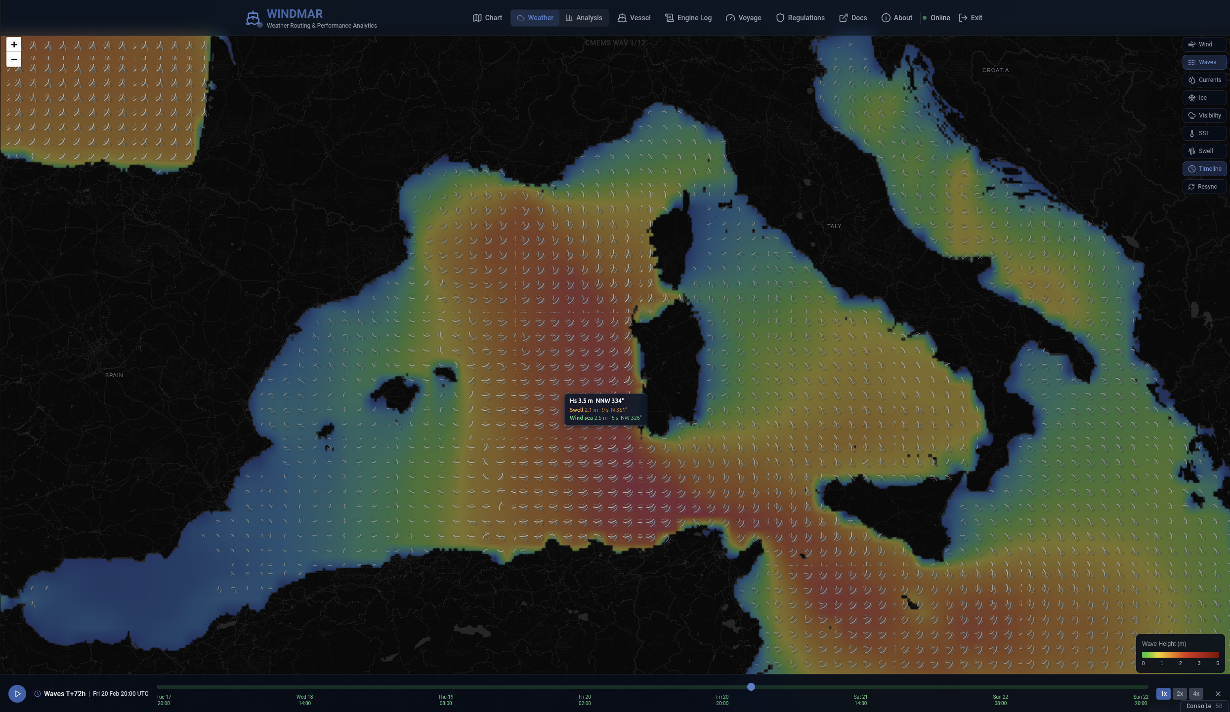
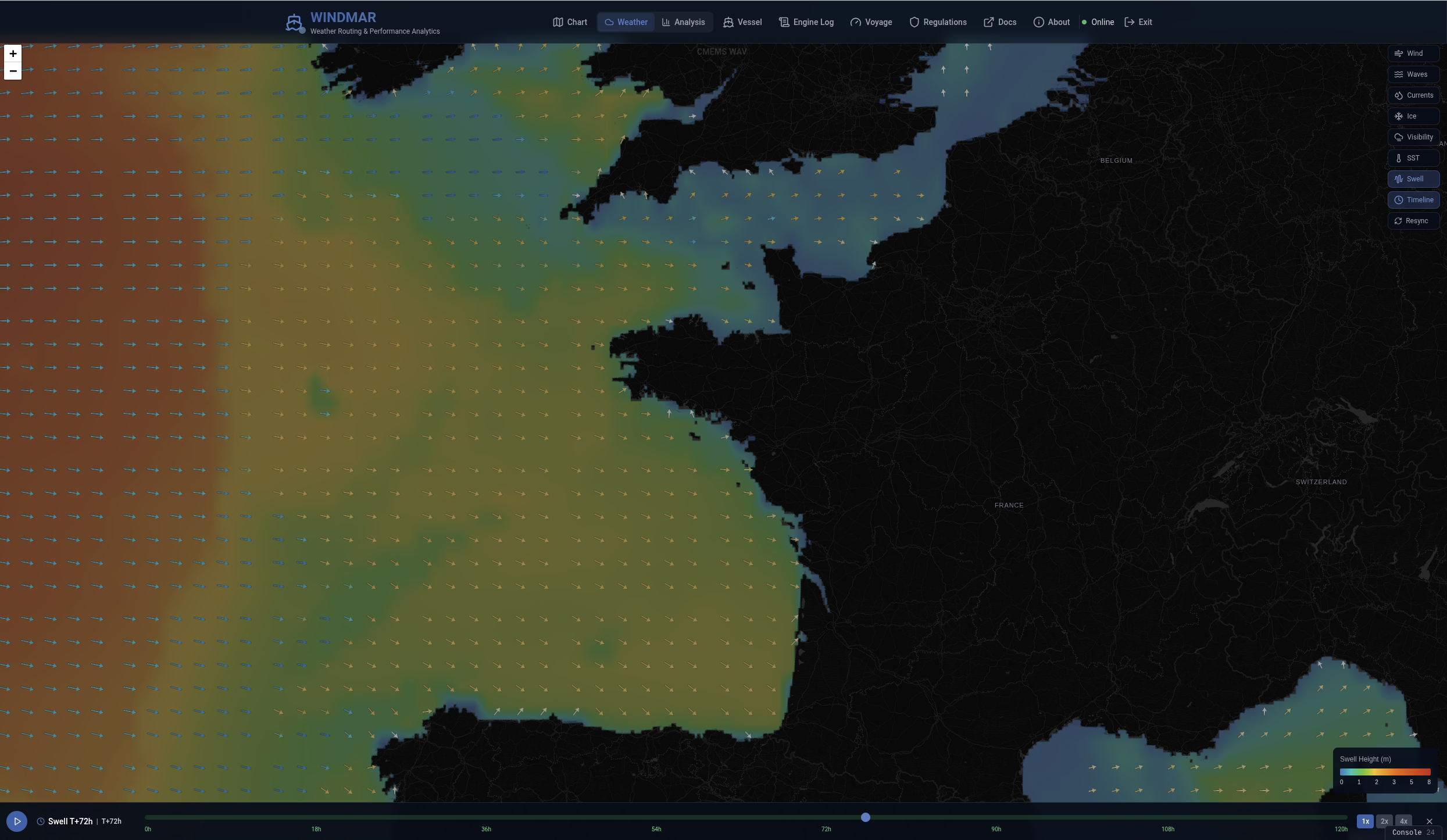
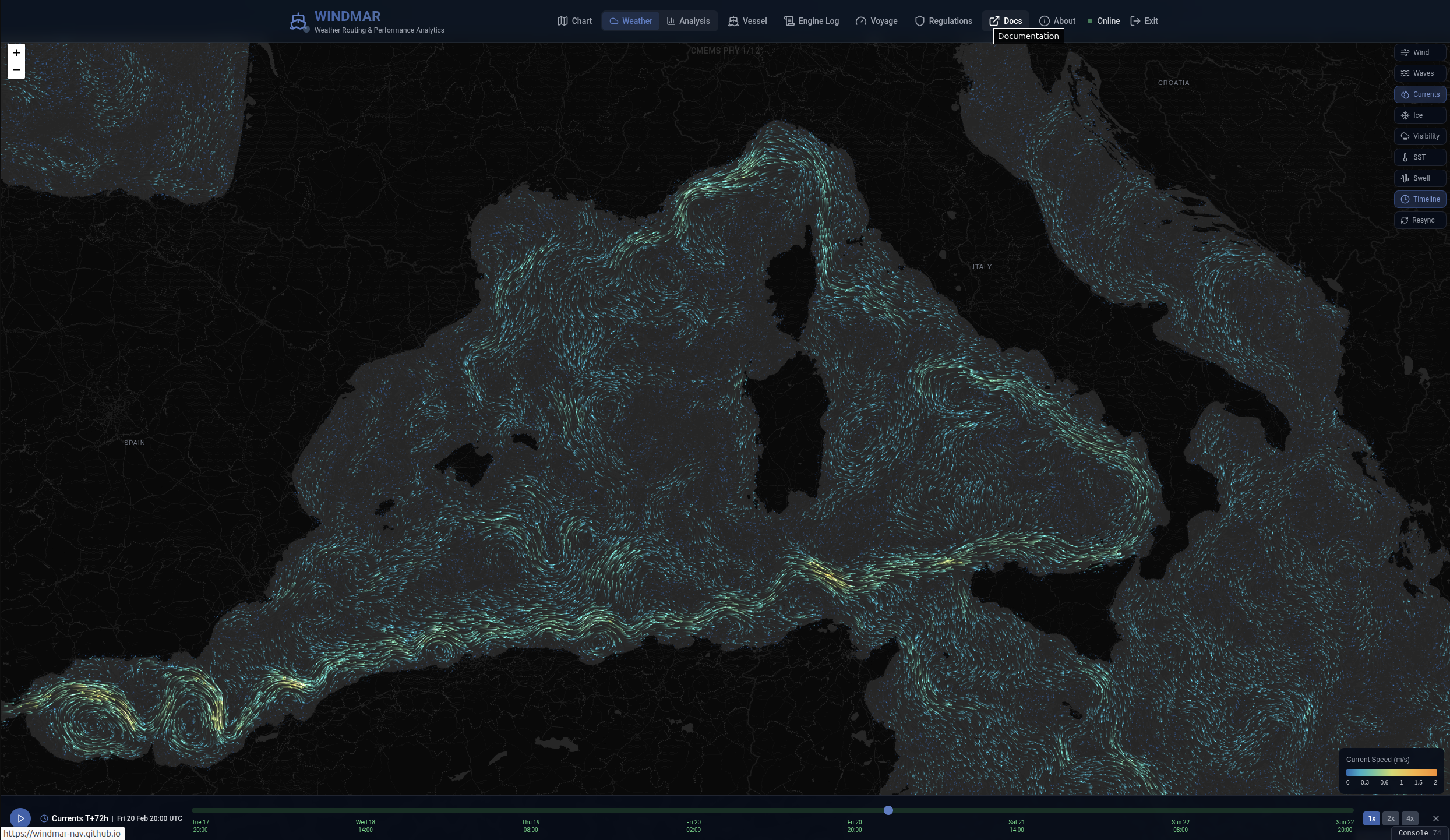
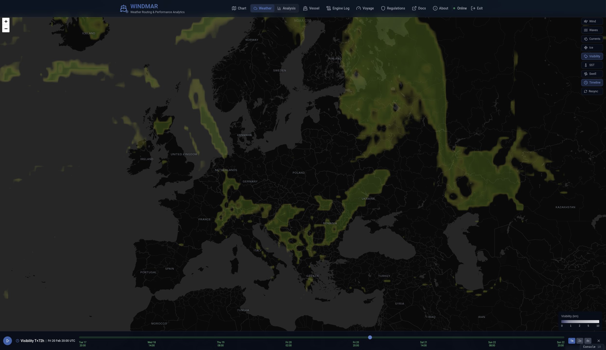
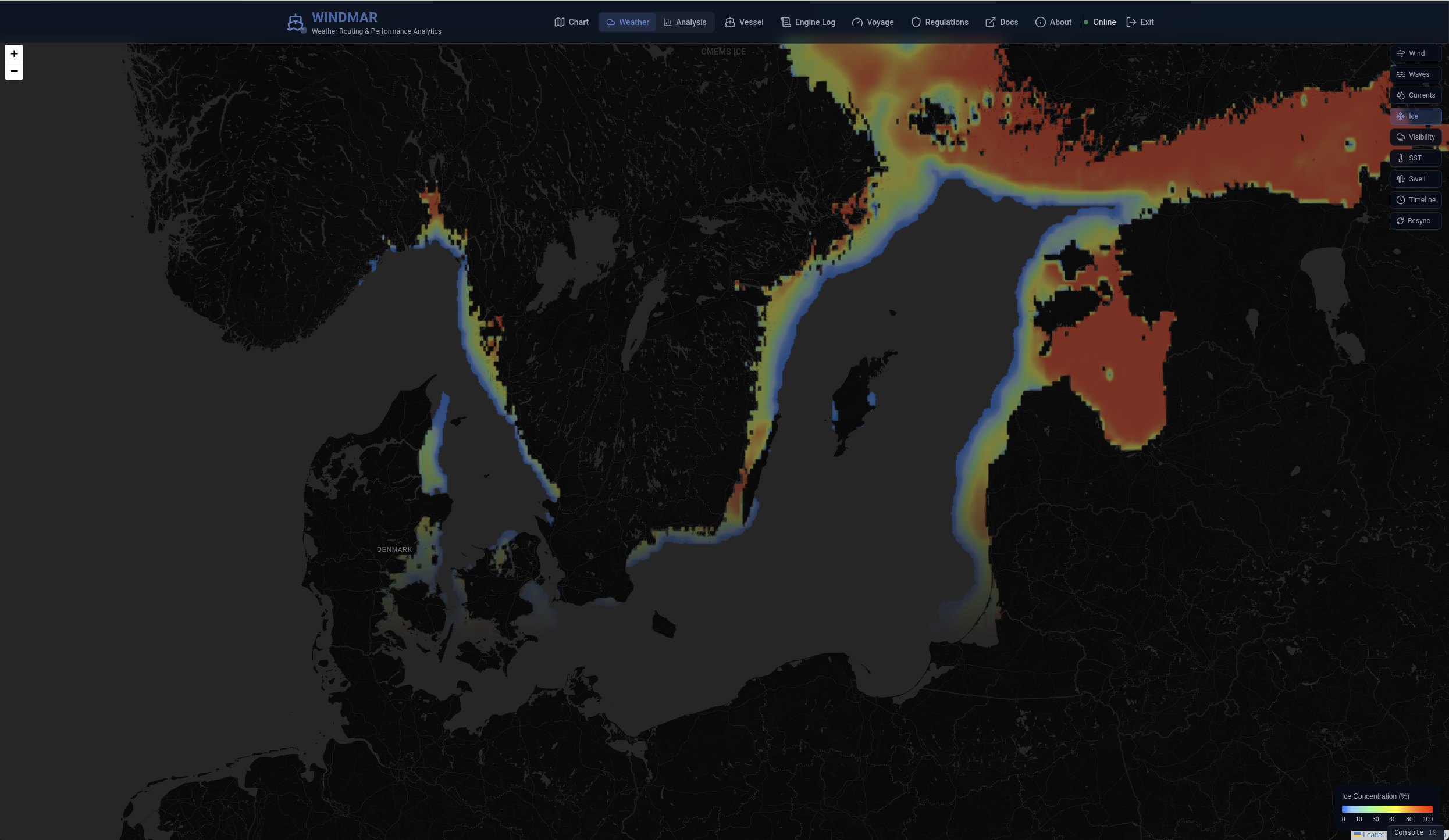
Baltic Ice Animation
Baltic Sea Ice Forecast — 5-day ice concentration animation showing ice coverage evolution across forecast timesteps
Route Optimization
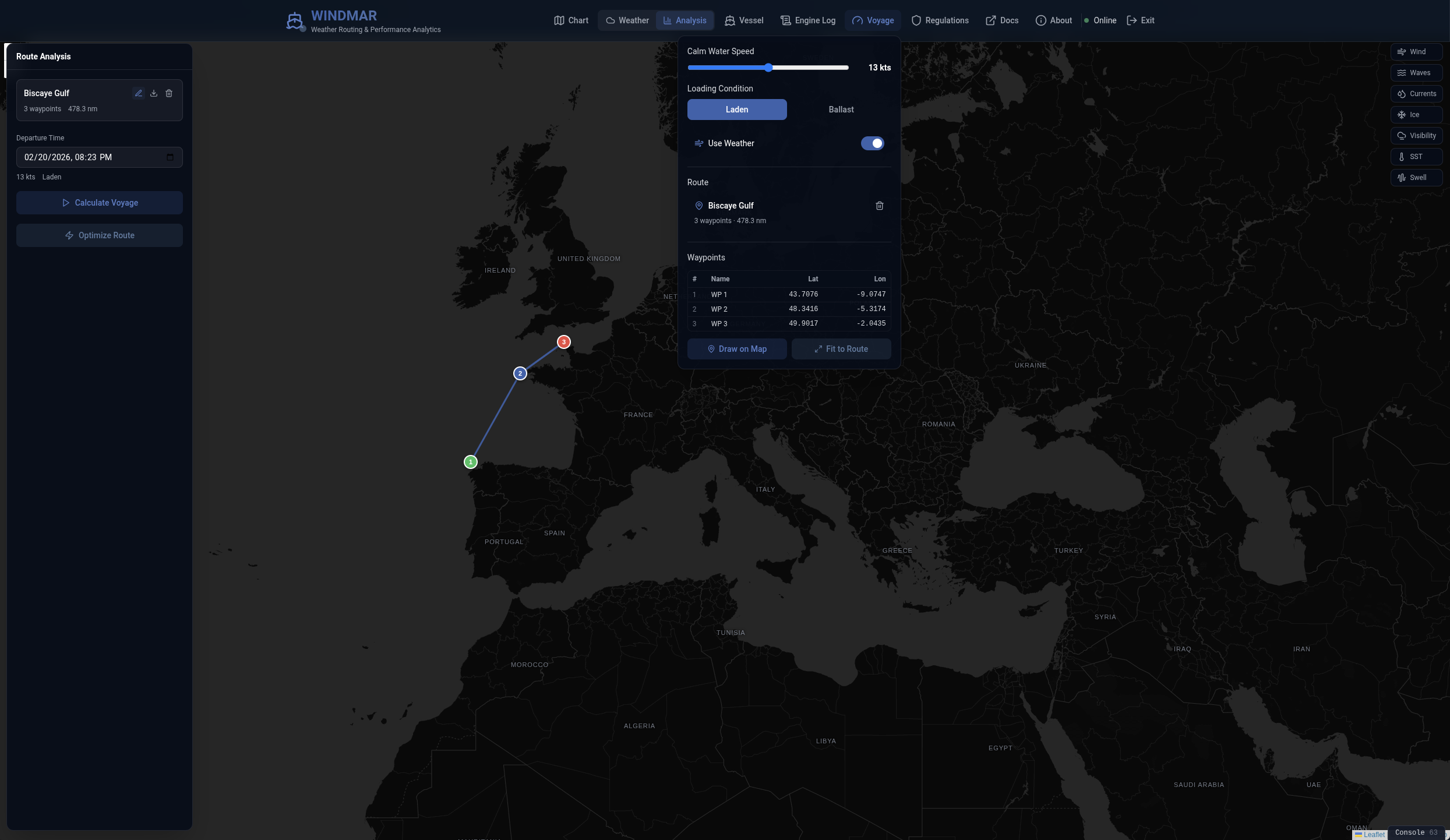
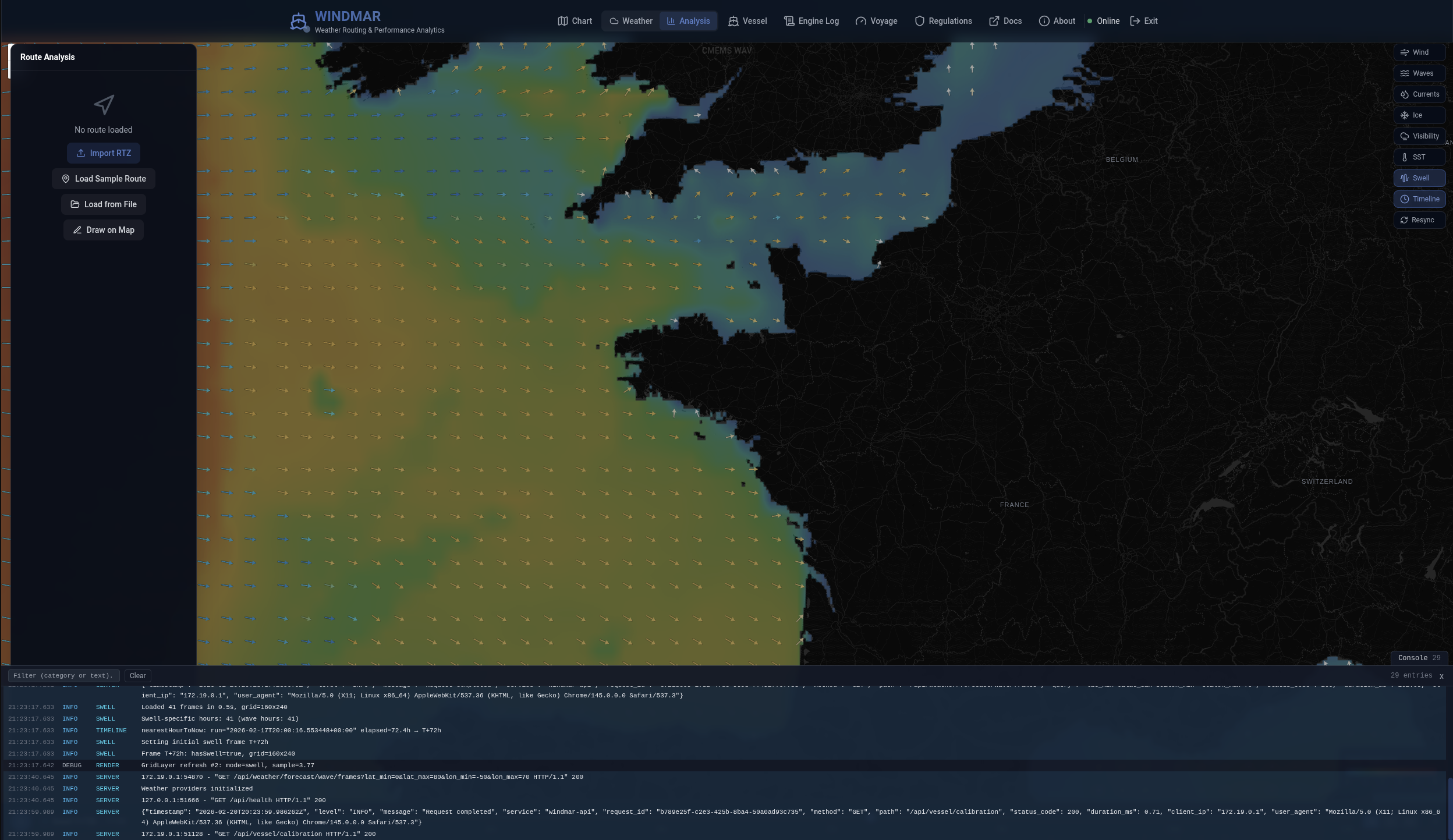
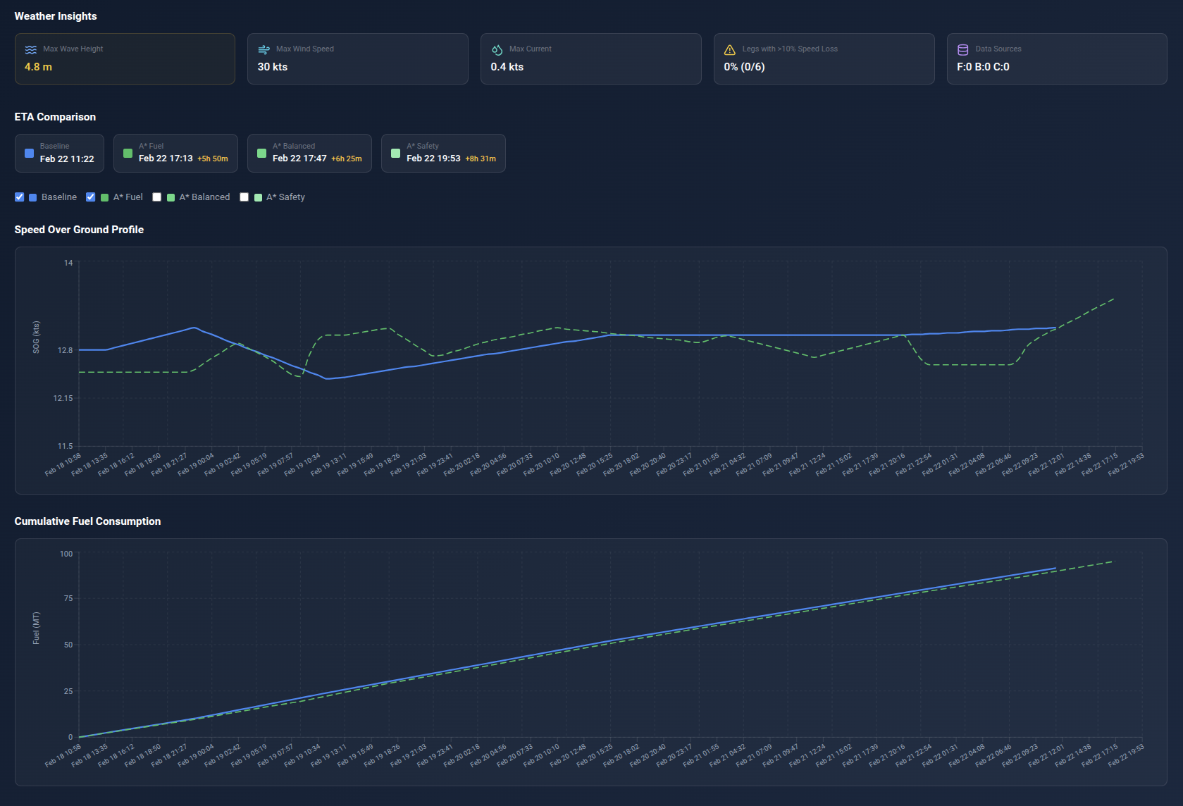
Vessel Performance
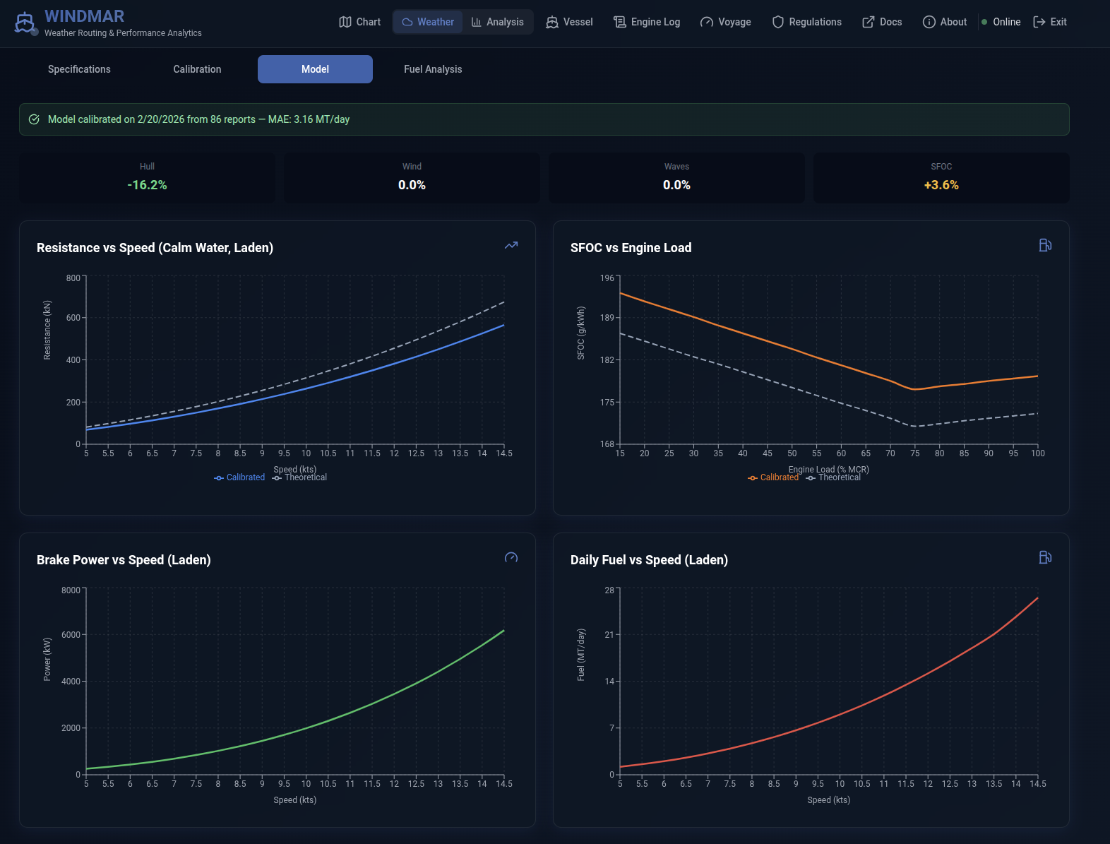
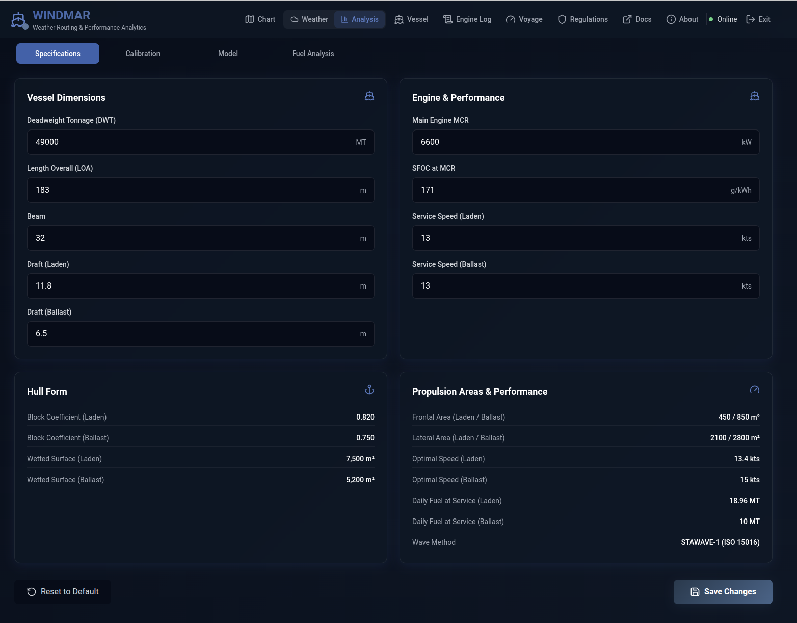
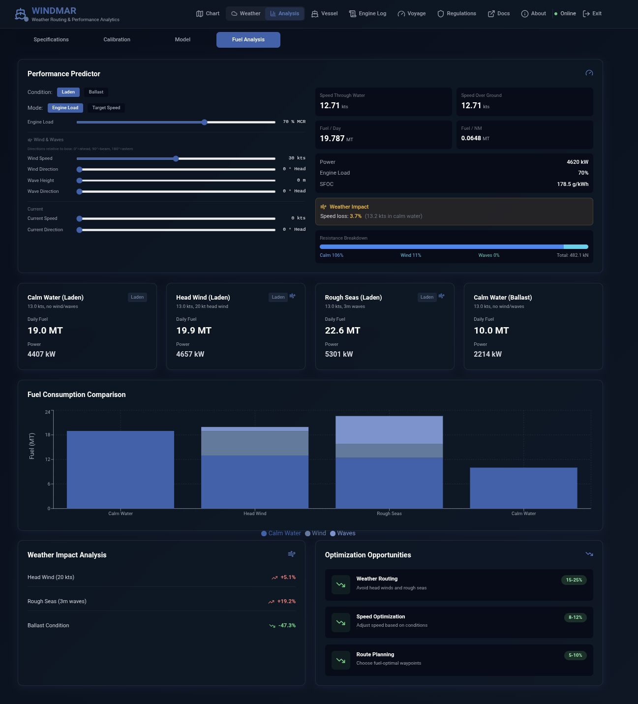
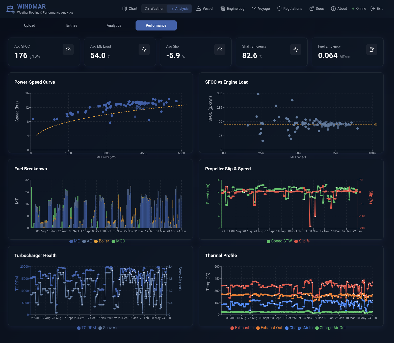
Engine Log & Compliance
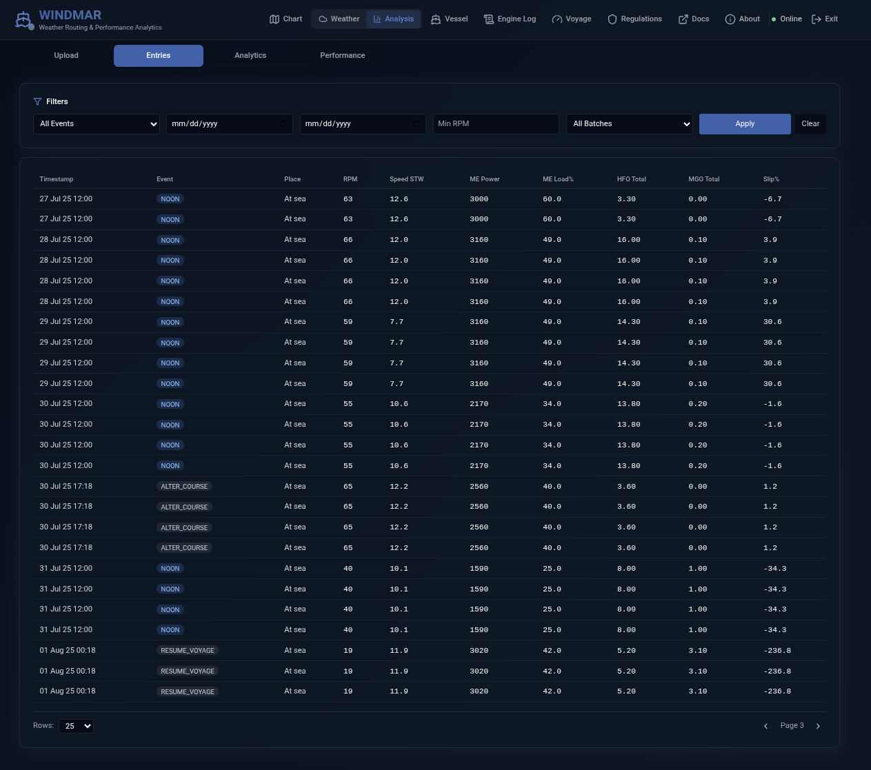
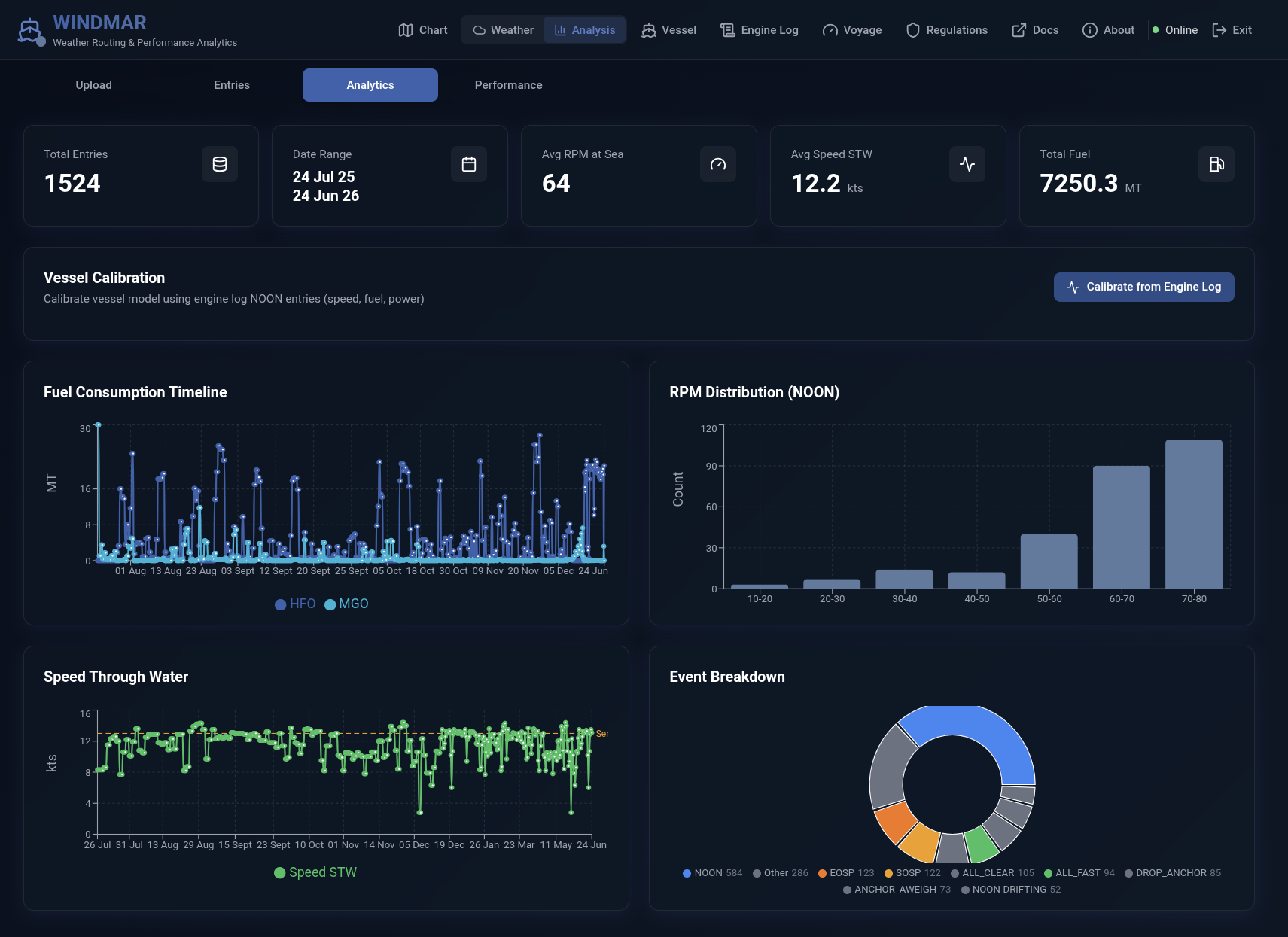
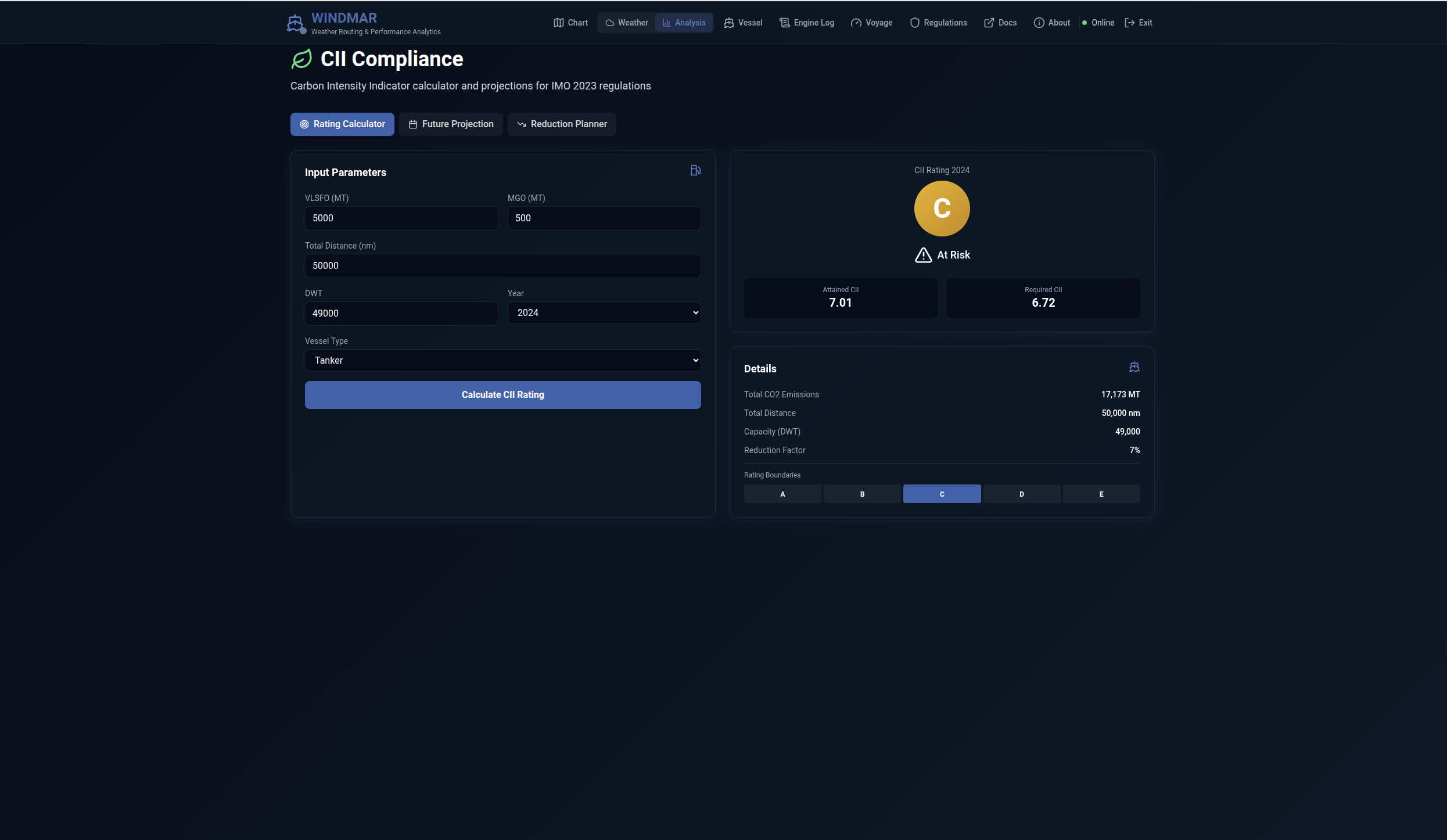
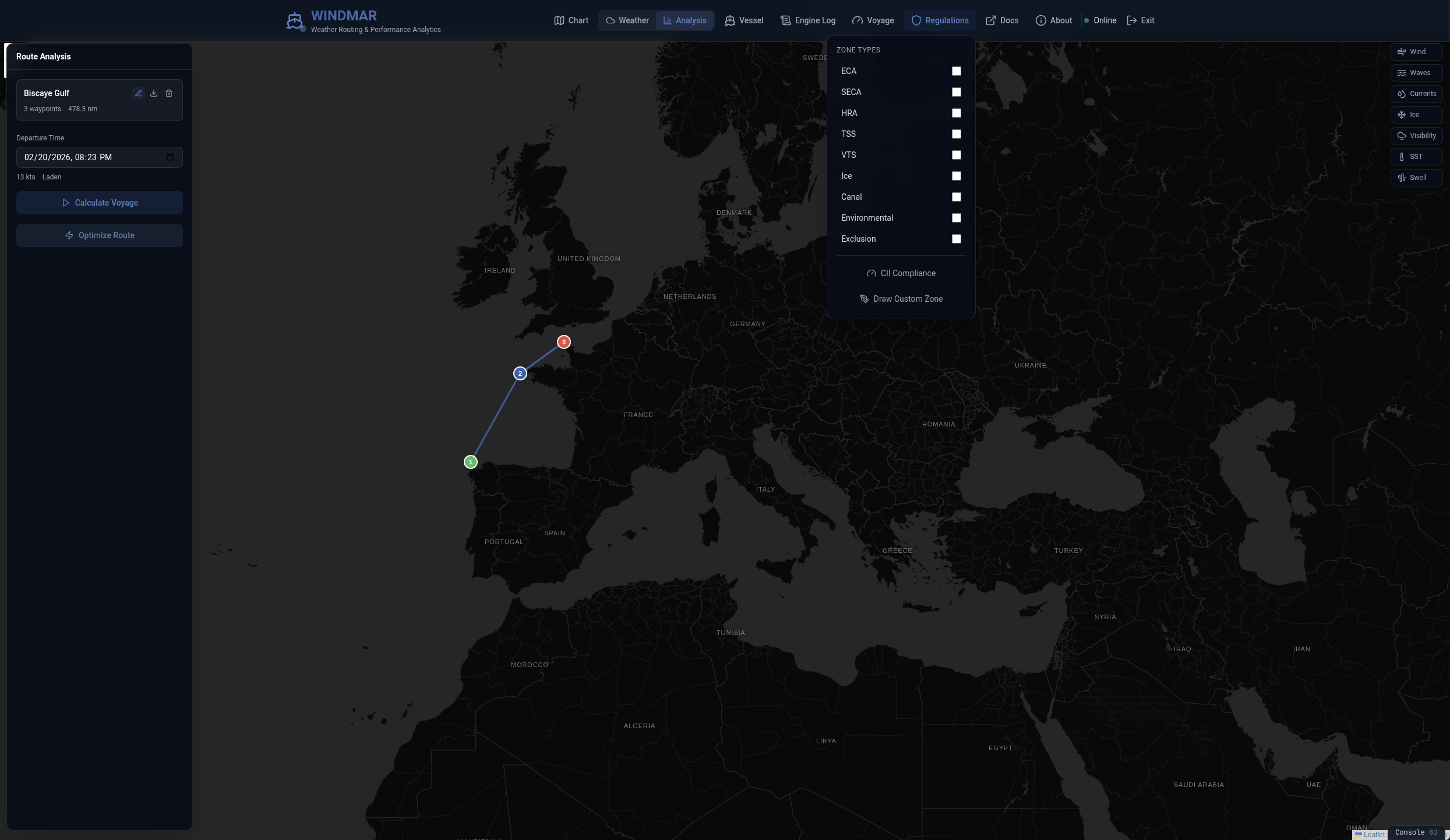
Technical Articles
The following peer-reviewed-style articles provide in-depth coverage of WindMar's core subsystems. Each article presents the mathematical foundations, implementation details, and relevant references for a specific domain of the weather routing pipeline.
Weather Data Fields
- Meteorological and oceanographic parameters: wind (GFS), waves (CMEMS), currents, and ocean masking used in vessel performance prediction.
Data Ingestion & Restitution
- Pipeline architecture from acquisition through compressed PostgreSQL storage to trilinear-interpolated, route-ready weather grids.
Hydrodynamics & RAO
- Holtrop-Mennen calm-water resistance, STAWAVE-1 added wave resistance, simplified RAO seakeeping, and noon-report calibration.
A* Pathfinding
- Adaptation of A* graph search to minimum-fuel ocean routing with physics-based cost evaluation and time-varying weather integration.
Weather Data Acquisition
- GFS and ERA5 wind data acquisition, CMEMS wave and current forecasts, and the unified forecast-climatology blending framework.
Monte Carlo Simulation
- Parametric Monte Carlo simulation with temporal weather correlation for voyage uncertainty quantification of fuel and ETA.
Trois problèmes ouverts
- Scénarios climatologiques par analogues Wasserstein, calibration spectrale du modèle navire, et stabilisation des trajectoires par splines contraintes. (Français)